Definitions and Basic Properties

Expected value is one of the most important concepts in probability. The expected value of a real-valued random variable gives the center of the distribution of the variable, in a special sense. Additionally, by computing expected values of various real transformations of a general random variable, we con extract a number of interesting characteristics of the distribution of the variable, including measures of spread, symmetry, and correlation. In a sense, expected value is a more general concept than probability itself.

Basic Concepts

Definitions

As usual, we start with a random experiment, modeled by a probability space

(Ω, F, P)

. So to review,

Ω

is the set of outcomes,

F

the collection of events, and

P

the probability measure on the sample space

(Ω, F)

. In the following definitions, we assume that

X

is a random variable for the experiment, with values in

S \subseteq R

Suppose that $X$ has a discrete distribution with probability density function $f$ . The expected value of $X$ is defined as follows (assuming that the sum is well defined): $E (X) = \sum_{x \in S} x f (x)$

Details

Recall that $S$ is countable and $f (x) = P (X = x)$ for $x \in S$ .

The sum defining the expected value makes sense if either the sum over the positive

x \in S

is finite or the sum over the negative

x \in S

is finite (or both). This ensures the that the entire sum exists (as an extended real number) and does not depend on the order of the terms. So as we will see, it's possible for

E (X)

to be a real number or

\infty

- \infty

or to simply not exist. Of course, if

S

is finite the expected value always exists as a real number.

Suppose that $X$ has a continuous distribution with probability density function $f$ . The expected value of $X$ is defined as follows (assuming that the integral is well defined): $E (X) = \int_{S} x f (x) d x$

Details:

In this case, $S$ is typically an interval or a union of disjoint intervals.

The probability density functions in basic applied probability that describe continuous distributions are piecewise continuous. So the integral above makes sense if the integral over positive

x \in S

is finite or the integral over negative

x \in S

is finite (or both). This ensures that the entire integral exists (as an extended real number). So as in the discrete case, it's possible for

E (X)

to exist as a real number or as

\infty

or as

- \infty

or to not exist at all. As you might guess, the definition for a mixed distribution is a combination of the definitions for the discrete and continuous cases.

Suppose that $X$ has a mixed distribution with partial discrete density $g$ on $D$ and partial continuous density $h$ on $C$ , where $D$ and $C$ are disjoint and $S = D \cup C$ . The expected value of $X$ is defined as follows (assuming that the expression on the right is well defined): $E (X) = \sum_{x \in D} x g (x) + \int_{C} x h (x) d x$

Details:

Recall that $D$ is countable and $C$ is typically an interval or a union of disjoint intervals.

For the expected value above to make sense, the sum must be well defined, as in the discrete case, the integral must be well defined, as in the continuous case, and we must avoid the dreaded indeterminate form

\infty - \infty

. As we will see in later, the various definitions given here can be unified into a single definition that works regardless of the type of distribution of

X

. An even more general definition can be given in terms of integrals.

Interpretation

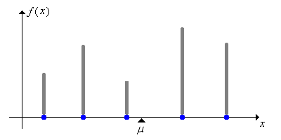
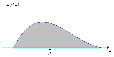
The expected value of

X

is also called the mean of the distribution of

X

and is frequently denoted

μ

. The mean is the center of the probability distribution of

X

in a special sense. Indeed, if we think of the distribution as a mass distribution (with total mass 1), then the mean is the center of mass as defined in physics. The two pictures below show discrete and continuous probability density functions; in each case the mean

μ

is the center of mass, the balance point.

To understand expected value in a probabilistic way, suppose that we create a new, compound experiment by repeating the basic experiment over and over again. This gives a sequence of independent random variables

(X_{1}, X_{2}, \dots)

, each with the same distribution as

X

. In statistical terms, we are sampling from the distribution of

X

. The average value, or sample mean, after

n

runs is

M_{n} = \frac{1}{n} \sum_{i = 1}^{n} X_{i}

Note that

M_{n}

is a random variable in the compound experiment. The important fact is that the average value

M_{n}

converges to the expected value

E (X)

n \to \infty

. The precise statement of this is the law of large numbers, one of the fundamental theorems of probability. You will see the law of large numbers at work in many of the simulation exercises given below.

Extensions

If $a \in R$ and $n \in N$ , the moment of $X$ about $a$ of order $n$ is defined to be $E [(X - a)^{n}]$ (assuming of course that this expected value exists).

The moments about 0 are simply referred to as moments (or sometimes raw moments). The moments about

μ

are the central moments. The second central moment is particularly important, and is known as the variance. In some cases, if we know all of the moments of

X

, we can determine the entire distribution of

X

. This idea is explored in the discussion of generating functions.

The expected value of a random variable

X

is based, of course, on the probability measure

P

for the experiment. This probability measure could be a conditional probability measure, conditioned on a given event

A \in F

with

P (A) > 0

. The usual notation is

E (X ∣ A)

, and this expected value is computed by the definitions given above, except that the conditional probability density function

x \mapsto f (x ∣ A)

replaces the ordinary probability density function

f

. It is very important to realize that, except for notation, no new concepts are involved. All results that we obtain for expected value in general have analogues for these conditional expected values. On the other hand, in a later section we will study a more general notion of conditional expected value.

Basic Properties

The purpose of this subsection is to study some of the essential properties of expected value. Unless otherwise noted, we will assume that the indicated expected values exist, and that the various sets and functions that we use are measurable. We start with two simple but still essential results.

Simple Variables

First, recall that a constant

c \in R

can be thought of as a random variable (on any probability space) that takes only the value

c

with probability 1. The corresponding distribution is sometimes called point mass at

c

If $c$ is a constant random variable, then $E (c) = c$ .

Details:

As a random variable, $c$ has a discrete distribution, so $E (c) = c \cdot 1 = c$ .

Next recall that an indicator variable is a random variable that takes only the values 0 and 1.

If $X$ is an indicator variable then $E (X) = P (X = 1)$ .

Details:

$X$ is discrete so by definition, $E (X) = 1 \cdot P (X = 1) + 0 \cdot P (X = 0) = P (X = 1)$ .

In particular, if

1_{A}

is the indicator variable of an event

A

, then

E (1_{A}) = P (A)

, so in a sense, expected value subsumes probability. For a book that takes expected value, rather than probability, as the fundamental starting concept, see Probability via Expectation, by Peter Whittle.

Change of Variables Theorem

The expected value of a real-valued random variable gives the center of the distribution of the variable. This idea is much more powerful than might first appear. By finding expected values of various functions of a general random variable, we can measure many interesting features of its distribution.

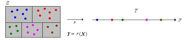
So, suppose that

X

is a random variable with values in a general set

S

, and suppose that

r

is a function from

S

into

R

. Then

r (X)

is a real-valued random variable, and so it makes sense to compute

E [r (X)]

(assuming as usual that this expected value exists). However, to compute this expected value from the definition would require that we know the probability density function of the transformed variable

r (X)

, a difficult problem in general. Fortunately, there is a much better way, given by the change of variables theorem for expected value. This theorem is sometimes referred to as the law of the unconscious statistician, presumably because it is so basic and natural that it is often used without the realization that it is a theorem, and not a definition.

If $X$ has a discrete distribution on a countable set $S$ with probability density function $f$ . then $E [r (X)] = \sum_{x \in S} r (x) f (x)$

Details:

Let $Y = r (X)$ and let $T \subseteq R$ denote the range of $r$ . Then $T$ is countable so $Y$ has a discrete distribution. Thus $E (Y) = \sum_{y \in T} y P (Y = y) = \sum_{y \in T} y \sum_{x \in r^{- 1} {y}} f (x) = \sum_{y \in T} \sum_{x \in r^{- 1} {y}} r (x) f (x) = \sum_{x \in S} r (x) f (x)$

The next result is the change of variables theorem when

X

has a continuous distribution. We will prove the continuous version in stages, first when

r

has discrete range below and then in the next section in full generality. Even though the complete proof is delayed, however, we will use the change of variables theorem in the proofs of many of the other properties of expected value.

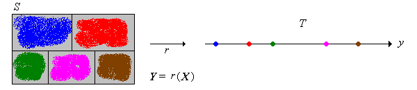
Suppose that $X$ has a continuous distribution on $S \subseteq R^{n}$ with probability density function $f$ , and that $r : S \to R$ . Then $E [r (X)] = \int_{S} r (x) f (x) d x$

Details:

Suppose that $r$ has discrete range and let $T$ denote the set of values of $Y = r (X)$ . By assumption, $T$ is countable so $Y$ has a discrete distribution. Thus $E (Y) = \sum_{y \in T} y P (Y = y) = \sum_{y \in T} y \int_{r^{- 1} {y}} f (x) d x = \sum_{y \in T} \int_{r^{- 1} {y}} r (x) f (x) d x = \int_{S} r (x) f (x) d x$

The results below gives basic properties of expected value. These properties are true in general, but we will restrict the proofs primarily to the continuous case. The proofs for the discrete case are analogous, with sums replacing integrals. The change of variables theorem is the main tool we will need. In these theorems

X

and

Y

are real-valued random variables for an experiment (that is, defined on an underlying probability space) and

c

is a constant. As usual, we assume that the indicated expected values exist. Be sure to try the proofs yourself before reading the ones in the text.

Linearity

$E (X + Y) = E (X) + E (Y)$

Details:

We apply the change of variables [8] with the function $r (x, y) = x + y$ . Suppose that $(X, Y)$ has a continuous distribution with PDF $f$ , and that $X$ takes values in $S \subseteq R$ and $Y$ takes values in $T \subseteq R$ . Recall that $X$ has PDF $g$ given by $g (x) = \int_{T} f (x, y) d y$ for $x \in S$ and $Y$ has PDF $h$ given by $h (y) = \int_{S} f (x, y) d x$ for $y \in T$ . Thus $\begin{aligned} E (X + Y) & = \int_{S \times T} (x + y) f (x, y) d (x, y) = \int_{S \times T} x f (x, y) d (x, y) + \int_{S \times T} y f (x, y) d (x, y) \\ = \int_{S} x (\int_{T} f (x, y) d y) d x + \int_{T} y (\int_{S} f (x, y) d x) d y = \int_{S} x g (x) d x + \int_{T} y h (y) d y = E (X) + E (Y) \end{aligned}$ Writing the double integrals as iterated integrals is a special case of Fubini's theorem. The proof in the discrete case is the same, with sums replacing integrals.

$E (c X) = c E (X)$

Details:

We apply the change of variables [8] with the function $r (x) = c x$ . Suppose that $X$ has a continuous distribution on $S \subseteq R$ with PDF $f$ . Then $E (c X) = \int_{S} c x f (x) d x = c \int_{S} x f (x) d x = c E (X)$ Again, the proof in the discrete case is the same, with sums replacing integrals.

Here is the linearity of expected value in full generality. It's a simple corollary of [9] and [10].

Suppose that $(X_{1}, X_{2}, \dots, X_{n})$ is a sequence of real-valued random variables defined on the underlying probability space and that $(a_{1}, a_{2}, \dots, a_{n})$ is a sequence of constants. Then $E (\sum_{i = 1}^{n} a_{i} X_{i}) = \sum_{i = 1}^{n} a_{i} E (X_{i})$

Thus, expected value is a linear operation on the collection of real-valued random variables for the experiment. The linearity of expected value is so basic that it is important to understand this property on an intuitive level. Indeed, it is implied by the interpretation of expected value given in the law of large numbers.

Suppose that $(X_{1}, X_{2}, \dots, X_{n})$ is a sequence of real-valued random variables with common mean $μ$ .

Let $Y = \sum_{i = 1}^{n} X_{i}$ , the sum of the variables. Then $E (Y) = n μ$ .
Let $M = \frac{1}{n} \sum_{i = 1}^{n} X_{i}$ , the average of the variables. Then $E (M) = μ$ .

Details:

By the additive property [9], $E (Y) = E (\sum_{i = 1}^{n} X_{i}) = \sum_{i = 1}^{n} E (X_{i}) = \sum_{i = 1}^{n} μ = n μ$
Note that $M = Y / n$ . Hence from the scaling property [10] and part (a), $E (M) = E (Y) / n = μ$ .

If the random variables in [12] are also independent and identically distributed, then in statistical terms, the sequence is a random sample of size

n

from the common distribution, and

M

is the sample mean.

In several important cases, a random variable from a special distribution can be decomposed into a sum of simpler random variables, and then part (a) of [12] can be used to compute the expected value.

Inequalities

The following results give some basic inequalities for expected value. The first, known as the positive property is the most obvious, but is also the main tool for proving the others.

Suppose that $P (X \geq 0) = 1$ . Then

$E (X) \geq 0$
If $P (X > 0) > 0$ then $E (X) > 0$ .

Details:

This result follows from the definition, since we can take the set of values $S$ of $X$ to be a subset of $[0, \infty)$ .
Suppose that $P (X > 0) > 0$ (in addition to $P (X \geq 0) = 1$ ). By the continuity theorem for increasing events, there exists $ϵ > 0$ such that $P (X \geq ϵ) > 0$ . Therefore $X - ϵ 1 (X \geq ϵ) \geq 0$ (with probability 1). By part (a), linearity, and Theorem 2, $E (X) - ϵ P (X \geq ϵ) > 0$ so $E (X) \geq ϵ P (X \geq ϵ) > 0$ .

Next is the increasing property, perhaps the most important property of expected value, after linearity.

Suppose that $P (X \leq Y) = 1$ . Then

$E (X) \leq E (Y)$
If $P (X < Y) > 0$ then $E (X) < E (Y)$ .

Details:

The assumption is equivalent to $P (Y - X \geq 0) = 1$ . Thus $E (Y - X) \geq 0$ by part (a) of the positive property [13]. But then $E (Y) - E (X) \geq 0$ by the linearity of expected value.
Similarly, this result follows from part (b) of the positive property [13].

Absolute value inequalities:

$| E (X) | \leq E (| X |)$
If $P (X > 0) > 0$ and $P (X < 0) > 0$ then $| E (X) | < E (| X |)$ .

Details:

Note that $- | X | \leq X \leq | X |$ (with probability 1) so by part (a) of the increasing property [14], $E (- | X |) \leq E (X) \leq E (| X |)$ . By linearity, $- E (| X |) \leq E (X) \leq E (| X |)$ which implies $| E (X) | \leq E (| X |)$ .
If $P (X > 0) > 0$ then $P (- | X | < X) > 0$ , and if $P (X < 0) > 0$ then $P (X < | X |) > 0$ . Hence by part (b) of the increasing property [14], $- E (| X |) < E (X) < E (| X |)$ and therefore $| E (X) | < E (| X |)$ .

If $P [X \neq E (X)] > 0$ then

$P [X > E (X)] > 0$
$P [X < E (X)] > 0$

Details:

We prove the contrapositive. Thus suppose that $P [X > E (X)] = 0$ so that $P [X \leq E (X)] = 1$ . If $P [X < E (X)] > 0$ then by the increasing property [14] we have $E (X) < E (X)$ , a contradiction. Thus $P [X = E (X)] = 1$ .
Similarly, if $P [X < E (X)] = 0$ then $P [X = E (X)] = 1$ .

Thus, if

X

is not a constant (with probability 1), then

X

must take values greater than its mean with positive probability and values less than its mean with positive probability.

Symmetry

Again, suppose that

X

is a random variable taking values in

R

. The distribution of

X

is symmetric about

a \in R

if the distribution of

a - X

is the same as the distribution of

X - a

Suppose that the distribution of $X$ is symmetric about $a \in R$ . If $E (X)$ exists, then $E (X) = a$ .

Details:

By assumption, the distribution of $X - a$ is the same as the distribution of $a - X$ . Since $E (X)$ exists we have $E (a - X) = E (X - a)$ so by linearity $a - E (X) = E (X) - a$ . Equivalently $2 E (X) = 2 a$ .

The previous result applies if

X

has a continuous distribution on

R

with a probability density

f

that is symmetric about

a

; that is,

f (a + x) = f (a - x)

for

x \in R

Independence

If $X$ and $Y$ are independent real-valued random variables then $E (X Y) = E (X) E (Y)$ .

Details:

Suppose that $X$ has a continuous distribution on $S \subseteq R$ with PDF $g$ and that $Y$ has a continuous distribution on $T \subseteq R$ with PDF $h$ . Then $(X, Y)$ has PDF $f (x, y) = g (x) h (y)$ on $S \times T$ . We apply the change of variables [8] with the function $r (x, y) = x y$ . $E (X Y) = \int_{S \times T} x y f (x, y) d (x, y) = \int_{S \times T} x y g (x) h (y) d (x, y) = \int_{S} x g (x) d x \int_{T} y h (y) d y = E (X) E (Y)$ The proof in the discrete case is similar with sums replacing integrals.

It follows from [18] that independent random variables are uncorrelated. Moreover, this result is more powerful than might first appear. Suppose that

X

and

Y

are independent random variables taking values in general sets

S

and

T

respectively, and that

u : S \to R

and

v : T \to R

. Then

u (X)

and

v (Y)

are independent, real-valued random variables and hence

E [u (X) v (Y)] = E [u (X)] E [v (Y)]

Examples and Applications

As always, be sure to try the proofs and computations yourself before reading the proof and answers in the text.

Uniform Distributions

Discrete uniform distributions are widely used in combinatorial probability, and model a point chosen at random from a finite set.

Suppose that $X$ has the discrete uniform distribution on a finite set $S \subseteq R$ .

$E (X)$ is the arithmetic average of the numbers in $S$ .
If the points in $S$ are evenly spaced with endpoints $a, b$ , then $E (X) = \frac{a + b}{2}$ , the average of the endpoints.

Details:

Let $n = # (S)$ , the number of points in $S$ . Then $X$ has PDF $f (x) = 1 / n$ for $x \in S$ so $E (X) = \sum_{x \in S} x \frac{1}{n} = \frac{1}{n} \sum_{x \in S} x$
Suppose that $S = {a, a + h, a + 2 h, \dots a + (n - 1) h}$ and let $b = a + (n - 1) h$ , the right endpoint. As in (a), $S$ has $n$ points so using (a) and the formula for the sum of the first $n - 1$ positive integers, we have $E (X) = \frac{1}{n} \sum_{i = 0}^{n - 1} (a + i h) = \frac{1}{n} (n a + h \frac{(n - 1) n}{2}) = a + \frac{(n - 1) h}{2} = \frac{a + b}{2}$

The results in [19] are easy to see if we think of

E (X)

as the center of mass, since the discrete uniform distribution corresponds to a finite set of points with equal mass.

Open the special distribution simulator, and select the discrete uniform distribution. This is the uniform distribution on $n$ points, starting at $a$ , evenly spaced at distance $h$ . Vary the parameters and note the location of the mean in relation to the probability density function. For selected values of the parameters, run the simulation 1000 times and compare the empirical mean to the distribution mean.

Recall that the continuous uniform distribution on a bounded interval corresponds to selecting a point at random from the interval. Continuous uniform distributions arise in geometric probability models and in a variety of other applied problems.

Suppose that $X$ has the continuous uniform distribution on an interval $[a, b]$ , where $a, b \in R$ and $a < b$ .

$E (X) = \frac{a + b}{2}$ , the midpoint of the interval.
$E (X^{n}) = \frac{1}{n + 1} (a^{n} + a^{n - 1} b + \dots + a b^{n - 1} + b^{n})$ for $n \in N$ .

Details:

Recall that $X$ has PDF $f (x) = \frac{1}{b - a}$ . Hence $E (X) = \int_{a}^{b} x \frac{1}{b - a} d x = \frac{1}{b - a} \frac{b^{2} - a^{2}}{2} = \frac{a + b}{2}$
By the change of variables [8], $E (X^{n}) = \int_{a}^{b} \frac{1}{b - a} x^{n} d x = \frac{b^{n + 1} - a^{n + 1}}{(n + 1) ‘ (b - a)} = \frac{1}{n + 1} (a^{n} + a^{n - 1} b + \dots a b^{n - 1} + b^{n})$

Part (a) is easy to see if we think of the mean as the center of mass, since the uniform distribution corresponds to a uniform distribution of mass on the interval.

Open the special distribution simulator, and select the continuous uniform distribution. This is the uniform distribution the interval $[a, a + w]$ . Vary the parameters and note the location of the mean in relation to the probability density function. For selected values of the parameters, run the simulation 1000 times and compare the empirical mean to the distribution mean.

Next, the average value of a function on an interval, as defined in calculus, has a nice interpretation in terms of the uniform distribution.

Suppose that $X$ is uniformly distributed on the interval $[a, b]$ , and that $g$ is an integrable function from $[a, b]$ into $R$ . Then $E [g (X)]$ is the average value of $g$ on $[a, b]$ : $E [g (X)] = \frac{1}{b - a} \int_{a}^{b} g (x) d x$

Details:

This result follows immediately from the change of variables [8], since $X$ has PDF $f (x) = 1 / (b - a)$ for $a \leq x \leq b$ .

Find the average value of the following functions on the given intervals:

$f (x) = x$ on $[2, 4]$
$g (x) = x^{2}$ on $[0, 1]$
$h (x) = \sin (x)$ on $[0, π]$ .

Details:

$3$
$\frac{1}{3}$
$\frac{2}{π}$

Exercise [25] given next illustrates the importance of the change of variables [8] in computing expected values.

Suppose that $X$ is uniformly distributed on $[- 1, 3]$ .

Give the probability density function of $X$ .
Find the probability density function of $X^{2}$ .
Find $E (X^{2})$ using the probability density function in (b).
Find $E (X^{2})$ using the change of variables [8].

Details:

$f (x) = \frac{1}{4}$ for $- 1 \leq x \leq 3$
$g (y) = {\begin{cases} \frac{1}{4} y^{- 1 / 2}, & 0 < y < 1 \\ \frac{1}{8} y^{- 1 / 2}, & 1 < y < 9 \end{cases}$
$\int_{0}^{9} y g (y) d y = \frac{7}{3}$
$\int_{- 1}^{3} x^{2} f (x) d x = \frac{7}{3}$

Dice

Recall that a standard die is a six-sided die. A fair die is one in which the faces are equally likely. An ace-six flat die is a standard die in which faces 1 and 6 have probability

\frac{1}{4}

each, and faces 2, 3, 4, and 5 have probability

\frac{1}{8}

each.

Two standard, fair dice are thrown, and the scores $(X_{1}, X_{2})$ recorded. Find the expected value of each of the following variables.

$Y = X_{1} + X_{2}$ , the sum of the scores.
$M = \frac{1}{2} (X_{1} + X_{2})$ , the average of the scores.
$Z = X_{1} X_{2}$ , the product of the scores.
$U = min {X_{1}, X_{2}}$ , the minimum score
$V = max {X_{1}, X_{2}}$ , the maximum score.

Details:

$7$
$\frac{7}{2}$
$\frac{49}{4}$
$\frac{91}{36}$
$\frac{161}{36}$

In the dice experiment, select two fair die. Note the shape of the probability density function and the location of the mean for the sum, minimum, and maximum variables. Run the experiment 1000 times and compare the sample mean and the distribution mean for each of these variables.

Two standard, ace-six flat dice are thrown, and the scores $(X_{1}, X_{2})$ recorded. Find the expected value of each of the following variables.

$Y = X_{1} + X_{2}$ , the sum of the scores.
$M = \frac{1}{2} (X_{1} + X_{2})$ , the average of the scores.
$Z = X_{1} X_{2}$ , the product of the scores.
$U = min {X_{1}, X_{2}}$ , the minimum score
$V = max {X_{1}, X_{2}}$ , the maximum score.

Details:

$7$
$\frac{7}{2}$
$\frac{49}{4}$
$\frac{77}{32}$
$\frac{147}{32}$

In the dice experiment, select two ace-six flat die. Note the shape of the probability density function and the location of the mean for the sum, minimum, and maximum variables. Run the experiment 1000 times and compare the sample mean and the distribution mean for each of these variables.

Bernoulli Trials

Recall that a Bernoulli trials process is a sequence

X = (X_{1}, X_{2}, \dots)

of independent, identically distributed indicator random variables. In the usual language of reliability,

X_{i}

denotes the outcome of trial

i

, where 1 denotes success and 0 denotes failure. The probability of success

p = P (X_{i} = 1) \in [0, 1]

is the basic parameter of the process. The process is named for Jacob Bernoulli.

For

n \in N_{+}

, the number of successes in the first

n

trials is

Y = \sum_{i = 1}^{n} X_{i}

. Recall that this random variable has the binomial distribution with parameters

n

and

p

, and has probability density function

f

given by

f (y) = (\binom{n}{y}) p^{y} (1 - p)^{n - y}, y \in {0, 1, \dots, n}

If $Y$ has the binomial distribution with parameters $n$ and $p$ then $E (Y) = n p$

Details:

We give two proofs. The first is from the definition. The critical tools that we need involve binomial coefficients: the identity $y (\binom{n}{y}) = n (\binom{n - 1}{y - 1})$ for $y, n \in N_{+}$ , and the binomial theorem $\begin{aligned} E (Y) & = \sum_{y = 0}^{n} y (\binom{n}{y}) p^{y} (1 - p)^{n - y} = \sum_{y = 1}^{n} n (\binom{n - 1}{y - 1}) p^{n} (1 - p)^{n - y} \\ = n p \sum_{y = 1}^{n - 1} (\binom{n - 1}{y - 1}) p^{y - 1} (1 - p)^{(n - 1) - (y - 1)} = n p [p + (1 - p)]^{n - 1} = n p \end{aligned}$

The second proof uses the additive property. Since $Y = \sum_{i = 1}^{n} X_{i}$ , the result follows immediately from and the additive property [9], since $E (X_{i}) = p$ for each $i \in N_{+}$ .

Note the superiority of the second proof to the first. The result also makes intuitive sense: in

n

trials with success probability

p

, we expect

n p

successes.

In the binomial coin experiment, vary $n$ and $p$ and note the shape of the probability density function and the location of the mean. For selected values of $n$ and $p$ , run the experiment 1000 times and compare the sample mean to the distribution mean.

Suppose that

p \in (0, 1]

, and let

N

denote the trial number of the first success. This random variable has the geometric distribution on

N_{+}

with parameter

p

, and has probability density function

g

given by

g (n) = p (1 - p)^{n - 1}, n \in N_{+}

If $N$ has the geometric distribution on $N_{+}$ with parameter $p \in (0, 1]$ then $E (N) = 1 / p$ .

Details:

The key is the formula for the deriviative of a geometric series: $E (N) = \sum_{n = 1}^{\infty} n p (1 - p)^{n - 1} = - p \frac{d}{d p} \sum_{n = 0}^{\infty} (1 - p)^{n} = - p \frac{d}{d p} \frac{1}{p} = p \frac{1}{p^{2}} = \frac{1}{p}$

Again, the result makes intuitive sense. Since

p

is the probability of success, we expect a success to occur after

1 / p

trials.

In the negative binomial experiment, select $k = 1$ to get the geometric distribution. Vary $p$ and note the shape of the probability density function and the location of the mean. For selected values of $p$ , run the experiment 1000 times and compare the sample mean to the distribution mean.

The Hypergeometric Distribution

Suppose that a population consists of

m

objects;

r

of the objects are type 1 and

m - r

are type 0. A sample of

n

objects is chosen at random, without replacement. The parameters

m, r, n \in N

with

r \leq m

and

n \leq m

. Let

X_{i}

denote the type of the

i

th object selected. Recall that

X = (X_{1}, X_{2}, \dots, X_{n})

is a sequence of identically distributed (but not independent) indicator random variable with

P (X_{i} = 1) = r / m

for each

i \in {1, 2, \dots, n}

Let

Y

denote the number of type 1 objects in the sample, so that

Y = \sum_{i = 1}^{n} X_{i}

. Recall that

Y

has the hypergeometric distribution, which has probability density function

f

given by

f (y) = \frac{(\binom{r}{y}) (\binom{m - r}{n - y})}{(\binom{m}{n})}, y \in {0, 1, \dots, n}

If $Y$ has the hypergeometric distribution with parameters $m$ , $n$ , and $r$ then $E (Y) = n \frac{r}{m}$ .

Details:

Our first proof is from the definition: Using the hypergeometric PDF, $E (Y) = \sum_{y = 0}^{n} y \frac{(\binom{r}{y}) (\binom{m - r}{n - y})}{(\binom{m}{n})}$ Note that the $y = 0$ term is 0. For the other terms, we can use the identity $y (\binom{r}{y}) = r (\binom{r - 1}{y - 1})$ to get $E (Y) = \frac{r}{(\binom{m}{n})} \sum_{y = 1}^{n} (\binom{r - 1}{y - 1}) (\binom{m - r}{n - y})$ But substituting $k = y - 1$ and using another fundamental identity, $\sum_{y = 1}^{n} (\binom{r - 1}{y - 1}) (\binom{m - r}{n - y}) = \sum_{k = 0}^{n - 1} (\binom{r - 1}{k}) (\binom{m - r}{n - 1 - k}) = (\binom{m - 1}{n - 1})$ So substituting and doing a bit of algebra gives $E (Y) = n \frac{r}{m}$ .

A much better proof uses [9] and the representation of $Y$ as a sum of indicator variables. The result follows immediately since $E (X_{i}) = r / m$ for each $i \in {1, 2, \dots n}$ .

In the ball and urn experiment, vary $n$ , $r$ , and $m$ and note the shape of the probability density function and the location of the mean. For selected values of the parameters, run the experiment 1000 times and compare the sample mean to the distribution mean.

Note that if we select the objects with replacement, then

X

would be a sequence of Bernoulli trials, and hence

Y

would have the binomial distribution with parameters

n

and

p = \frac{r}{m}

. Thus, the mean would still be

E (Y) = n \frac{r}{m}

The Poisson Distribution

Recall that the Poisson distribution has probability density function

f

given by

f (n) = e^{- a} \frac{a^{n}}{n!}, n \in N

where

a \in (0, \infty)

is a parameter. The Poisson distribution is named after Simeon Poisson and is widely used to model the number of random points in a region of time or space; the parameter

a

is proportional to the size of the region.

If $N$ has the Poisson distribution with parameter $a$ then $E (N) = a$ . Thus, the parameter of the Poisson distribution is the mean of the distribution.

Details:

The proof depends on the standard series for the exponential function

E (N) = \sum_{n = 0}^{\infty} n e^{- a} \frac{a^{n}}{n!} = e^{- a} \sum_{n = 1}^{\infty} \frac{a^{n}}{(n - 1)!} = e^{- a} a \sum_{n = 1}^{\infty} \frac{a^{n - 1}}{(n - 1)!} = e^{- a} a e^{a} = a .

In the Poisson experiment, the parameter is $a = r t$ . Vary the parameter and note the shape of the probability density function and the location of the mean. For various values of the parameter, run the experiment 1000 times and compare the sample mean to the distribution mean.

The Exponential Distribution

Recall that the exponential distribution is a continuous distribution with probability density function

f

given by

f (t) = r e^{- r t}, t \in [0, \infty)

where

r \in (0, \infty)

is the rate parameter. This distribution is widely used to model failure times and other arrival times; in particular, the distribution governs the time between arrivals in the Poisson model.

Suppose that $T$ has the exponential distribution with rate parameter $r$ . Then $E (T) = 1 / r$ .

Details:

This result follows from the definition and an integration by parts:

E (T) = \int_{0}^{\infty} t r e^{- r t} d t = - t e^{- r t} |_{0}^{\infty} + \int_{0}^{\infty} e^{- r t} d t = 0 - \frac{1}{r} e^{- r t} |_{0}^{\infty} = \frac{1}{r}

Recall that the mode of

T

is 0 and the median of

T

\ln 2 / r

. Note how these measures of center are ordered:

0 < \ln 2 / r < 1 / r

In the gamma experiment, set $n = 1$ to get the exponential distribution. This app simulates the first arrival in a Poisson process. Vary $r$ with the scrollbar and note the position of the mean relative to the graph of the probability density function. For selected values of $r$ , run the experiment 1000 times and compare the sample mean to the distribution mean.

Suppose again that $T$ has the exponential distribution with rate parameter $r$ and suppose that $t > 0$ . Find $E (T ∣ T > t)$ .

Details:

$t + \frac{1}{r}$

The Erlang Distribution

Recall that the Erlang distribution is a continuous distribution with probability density function

f

given by

f (t) = r^{n} \frac{t^{n - 1}}{(n - 1)!} e^{- r t}, t \in [0, \infty)

where

n \in N_{+}

is the shape parameter and

r \in (0, \infty)

is the rate parameter. This distribution is widely used to model failure times and other arrival times, and in particular, models the

n

th arrival in the Poisson process. So it follows that if

(X_{1}, X_{2}, \dots, X_{n})

is a sequence of independent random variables, each having the exponential distribution with rate parameter

r

, then

T = \sum_{i = 1}^{n} X_{i}

has the Erlang distribution with shape parameter

n

and rate parameter

r

. The Erlang distribution is a special case of the gamma distribution which allows non-integer shape parameters.

Suppose that $T$ has the Erlang distribution with shape parameter $n$ and rate parameter $r$ . Then $E (T) = n / r$ .

Details:

We give two proofs. The first is by induction on $n$ , so let $μ_{n}$ denote the mean when the shape parameter is $n \in N_{+}$ . When $n = 1$ , we have the exponential distribution with rate parameter $r$ , so we know $μ_{1} = 1 / r$ by [38]. Suppose that $μ_{n} = r / n$ for a given $n \in N_{+}$ . Then $μ_{n + 1} = \int_{0}^{\infty} t r^{n + 1} \frac{t^{n}}{n!} e^{- r t} d t = \int_{0}^{\infty} r^{n + 1} \frac{t^{n + 1}}{n!} e^{- r t} d t$ Integrate by parts with $u = \frac{t^{n + 1}}{n!}$ , $d v = r^{n + 1} e^{- r t} d t$ so that $d u = (n + 1) \frac{t^{n}}{n!} d t$ and $v = - r^{n} e^{- r t}$ . Then $μ_{n + 1} = (n + 1) \int_{0}^{\infty} r^{n} \frac{t^{n}}{n!} e^{- r t} d t = \frac{n + 1}{n} \int_{0}^{\infty} t r^{n} \frac{t^{n - 1}}{(n - 1)!} d t$ But the last integral is $μ_{n}$ , so by the induction hypothesis, $μ_{n + 1} = \frac{n + 1}{n} \frac{n}{r} = \frac{n + 1}{r}$ .

The second proof is much better. The result follows immediately from the additive property [9] and the fact that $T$ can be represented in the form $T = \sum_{i = 1}^{n} X_{i}$ where $X_{i}$ has the exponential distribution with parameter $r$ for each $i \in {1, 2, \dots, n}$ .

Note again how much easier and more intuitive the second proof is than the first.

Open the gamma experiment, which simulates the arrival times in the Poisson process. Vary the parameters and note the position of the mean relative to the graph of the probability density function. For selected parameter values, run the experiment 1000 times and compare the sample mean to the distribution mean.

Beta Distributions

The distributions in this subsection belong to the family of beta distributions, which are widely used to model random proportions and probabilities.

Suppose that $X$ has probability density function $f$ given by $f (x) = 3 x^{2}$ for $x \in [0, 1]$ .

Find the mean of $X$ .
Find the mode of $X$ .
Find the median of $X$ .
Sketch the graph of $f$ and show the location of the mean, median, and mode on the $x$ -axis.

Details:

$\frac{3}{4}$
$1$
${(\frac{1}{2})}^{1 / 3}$

In the special distribution simulator, select the beta distribution and set $a = 3$ and $b = 1$ to get the distribution in [43]. Run the experiment 1000 times and compare the sample mean to the distribution mean.

Suppose that a sphere has a random radius $R$ with probability density function $f$ given by $f (r) = 12 r^{2} (1 - r)$ for $r \in [0, 1]$ . Find the expected value of each of the following:

The circumference $C = 2 π R$
The surface area $A = 4 π R^{2}$
The volume $V = \frac{4}{3} π R^{3}$

Details:

$\frac{6}{5} π$
$\frac{8}{5} π$
$\frac{8}{21} π$

Suppose that $X$ has probability density function $f$ given by $f (x) = \frac{1}{π \sqrt{x (1 - x)}}$ for $x \in (0, 1)$ .

Find the mean of $X$ .
Find median of $X$ .
Note that $f$ is unbounded, so $X$ does not have a mode.
Sketch the graph of $f$ and show the location of the mean and median on the $x$ -axis.

Details:

$\frac{1}{2}$
$\frac{1}{2}$

The particular beta distribution in [46] is also known as the (standard) arcsine distribution. It governs the last time that the Brownian motion process hits 0 during the time interval

[0, 1]

Open the Brownian motion experiment and select the last zero. Run the simulation 1000 times and compare the sample mean to the distribution mean.

Suppose that the grades on a test are described by the random variable $Y = 100 X$ where $X$ has the beta distribution with probability density function $f$ given by $f (x) = 12 x (1 - x)^{2}$ for $x \in [0, 1]$ . The grades are generally low, so the teacher decides to curve the grades using the transformation $Z = 10 \sqrt{Y} = 100 \sqrt{X}$ . Find the expected value of each of the following variables

Details:

$E (X) = \frac{2}{5}$
$E (Y) = 40$
$E (Z) = \frac{1280}{21} \approx 60.95$

The Pareto Distribution

Recall that the Pareto distribution is a continuous distribution with probability density function

f

given by

f (x) = \frac{a}{x^{a + 1}}, x \in [1, \infty)

where

a \in (0, \infty)

is a parameter. The Pareto distribution is named for Vilfredo Pareto. It is a heavy-tailed distribution that is widely used to model certain financial variables.

Suppose that $X$ has the Pareto distribution with shape parameter $a$ . Then

$E (X) = \infty$ if $0 < a \leq 1$
$E (X) = \frac{a}{a - 1}$ if $a > 1$

Details:

If $0 < a < 1$ , $E (X) = \int_{1}^{\infty} x \frac{a}{x^{a + 1}} d x = \int_{1}^{\infty} \frac{a}{x^{a}} d x = \frac{a}{- a + 1} x^{- a + 1} |_{1}^{\infty} = \infty$ since the exponent $- a + 1 > 0$ . If $a = 1$ , $E (X) = \int_{1}^{\infty} x \frac{1}{x^{2}} d x = \int_{1}^{\infty} \frac{1}{x} d x = \ln x |_{1}^{\infty} = \infty$ .
If $a > 1$ then $E (X) = \int_{1}^{\infty} x \frac{a}{x^{a + 1}} d x = \int_{1}^{\infty} \frac{a}{x^{a}} d x = \frac{a}{- a + 1} x^{- a + 1} |_{1}^{\infty} = \frac{a}{a - 1}$

Exercise [49] gives us our first example of a distribution whose mean is infinite.

In the special distribution simulator, select the Pareto distribution. Note the shape of the probability density function and the location of the mean. For the following values of the shape parameter $a$ , run the experiment 1000 times and note the behavior of the empirical mean.

$a = 1$
$a = 2$
$a = 3$ .

The Cauchy Distribution

Recall that the (standard) Cauchy distribution has probability density function

f

given by

f (x) = \frac{1}{π (1 + x^{2})}, x \in R

This distribution is named for Augustin Cauchy.

If $X$ has the Cauchy distribution then $E (X)$ does not exist.

Details:

By definition, $E (X) = \int_{- \infty}^{\infty} x \frac{1}{π (1 + x^{2})} d x = \frac{1}{2 π} \ln (1 + x^{2}) |_{- \infty}^{\infty}$ which evaluates to the meaningless expression $\infty - \infty$ .

Note that the graph of

f

is symmetric about 0 and is unimodal, and so the mode and median of

X

are both 0. By the symmetry result [17], if

X

had a mean, the mean would be 0 also, but alas the mean does not exist. Moreover, the non-existence of the mean is not just a pedantic technicality. If we think of the probability distribution as a mass distribution, then the moment to the right of

a

\int_{a}^{\infty} (x - a) f (x) d x = \infty

and the moment to the left of

a

\int_{- \infty}^{a} (x - a) f (x) d x = - \infty

for every

a \in R

. The center of mass simply does not exist. Probabilisitically, the law of large numbers fails, as you can see in the following simulation exercise:

In the Cauchy experiment (with the default parameter values), a light sources is 1 unit from position 0 on an infinite straight wall. The angle that the light makes with the perpendicular is uniformly distributed on the interval $(\frac{- π}{2}, \frac{π}{2})$ , so that the position of the light beam on the wall has the Cauchy distribution. Run the simulation 1000 times and note the behavior of the empirical mean.

The Normal Distribution

Recall that the standard normal distribution is a continuous distribution with density function

ϕ

given by

ϕ (z) = \frac{1}{\sqrt{2 π}} e^{- \frac{1}{2} z^{2}}, z \in R

Normal distributions are widely used to model physical measurements subject to small, random errors.

If $Z$ has the standard normal distribution then $E (X) = 0$ .

Details:

Using a simple change of variables, we have $E (Z) = \int_{- \infty}^{\infty} z \frac{1}{\sqrt{2 π}} e^{- \frac{1}{2} z^{2}} d z = - \frac{1}{\sqrt{2 π}} e^{- \frac{1}{2} z^{2}} |_{- \infty}^{\infty} = 0 - 0$

The standard normal distribution is unimodal and symmetric about

0

, so the median, mean, and mode all agree. More generally, for

μ \in (- \infty, \infty)

and

σ \in (0, \infty)

, recall that

X = μ + σ Z

has the normal distribution with location parameter

μ

and scale parameter

σ

X

has probability density function

f

given by

f (x) = \frac{1}{\sqrt{2 π} σ} \exp [- \frac{1}{2} {(\frac{x - μ}{σ})}^{2}], x \in R

The location parameter is the mean of the distribution:

If $X$ has the normal distribution with location parameter $μ \in R$ and scale parameter $σ \in (0, \infty)$ , then $E (X) = μ$

Details:

Of course we could use the definition, but a proof using linearity in and the representation in terms of the standard normal distribution is trivial: $E (X) = μ + σ E (Z) = μ$ .

In the special distribution simulator, select the normal distribution. Vary the parameters and note the location of the mean. For selected parameter values, run the simulation 1000 times and compare the sample mean to the distribution mean.

Additional Exercises

Suppose that $(X, Y)$ has probability density function $f$ given by $f (x, y) = x + y$ for $(x, y) \in [0, 1] \times [0, 1]$ . Find the following expected values:

$E (X)$
$E (X^{2} Y)$
$E (X^{2} + Y^{2})$
$E (X Y ∣ Y > X)$

Details:

$\frac{7}{12}$
$\frac{17}{72}$
$\frac{5}{6}$
$\frac{1}{3}$

Suppose that $N$ has a discrete distribution with probability density function $f$ given by $f (n) = \frac{1}{50} n^{2} (5 - n)$ for $n \in {1, 2, 3, 4}$ . Find each of the following:

The median of $N$ .
The mode of $N$
$E (N)$ .
$E (N^{2})$
$E (1 / N)$ .
$E (1 / N^{2})$ .

Details:

3
3
$\frac{73}{25}$
$\frac{47}{5}$
$\frac{2}{5}$
$\frac{1}{5}$

Suppose that $X$ and $Y$ are real-valued random variables with $E (X) = 5$ and $E (Y) = - 2$ . Find $E (3 X + 4 Y - 7)$ .

Details:

Suppose that $X$ and $Y$ are real-valued, independent random variables, and that $E (X) = 5$ and $E (Y) = - 2$ . Find $E [(3 X - 4) (2 Y + 7)]$ .

Details:

Suppose that there are 5 duck hunters, each a perfect shot. A flock of 10 ducks fly over, and each hunter selects one duck at random and shoots. Find the expected number of ducks killed.

Details:

Number the ducks from 1 to 10. For $k \in {1, 2, \dots, 10}$ , let $X_{k}$ be the indicator variable that takes the value 1 if duck $k$ is killed and 0 otherwise. Duck $k$ is killed if at least one of the hunters selects her, so $E (X_{k}) = P (X_{k} = 1) = 1 - {(\frac{9}{10})}^{5}$ . The number of ducks killed is $N = \sum_{k = 1}^{10} X_{k}$ so $E (N) = 10 [1 - {(\frac{9}{10})}^{5}] = 4.095$

For a more complete analysis of the duck hunter problem is given in a separate section.

Consider the following game: An urn initially contains one red and one green ball. A ball is selected at random, and if the ball is green, the game is over. If the ball is red, the ball is returned to the urn, another red ball is added, and the game continues. At each stage, a ball is selected at random, and if the ball is green, the game is over. If the ball is red, the ball is returned to the urn, another red ball is added, and the game continues. Let $X$ denote the length of the game (that is, the number of selections required to obtain a green ball). Find $E (X)$ .

Details:

The probability density function $f$ of $X$ was found in in the section on discrete distributions: $f (x) = \frac{1}{x (x + 1)}$ for $x \in N_{+}$ . The expected length of the game is infinite: $E (X) = \sum_{x = 1}^{\infty} x \frac{1}{x (x + 1)} = \sum_{x = 1}^{\infty} \frac{1}{x + 1} = \infty$