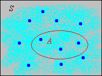
We have peviously studied discrete distributions and continuous distributions on Euclidean spaces. In this section, we will study probability measure that that are combinations of the two types.
\((\R^n, \ms R^n, \lambda^n)\) is the \(n\)-dimensional Euclidean measure space for \(n \in \N_+\), where \(\ms R^n\) is the \(\sigma\)-algebra of Borel measurable subsets of \(\R^n\) and \(\lambda^n\) is Lebesgue measure.
Our starting point in this section is a subspace \((S, \ms S)\) where \(S \in \ms R^n\) with \(\lambda^n(S) \gt 0\) and \(\ms S = \{A \in \ms R^n: A \subseteq S\}\).
A probability measure \(P\) on \(S\) is of mixed type if \(S\) can be partitioned into events \(D\) and \(C = D^c\) with the following properties:
Note that since \(D\) is countable, \(D \in \ms S\) and hence \(C \in \ms S\), so the definition makes sense.
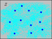
Thus, part of the distribution is concentrated at points in a discrete set \(D\); the rest of the distribution is continuously spread over \(C\). In the picture below, the light blue shading is intended to represent a continuous distribution of probability while the darker blue dots are intended to represents points of positive probability. The points in \(D\) are the atoms of the distribution.

Let \(\ms D\) denote the collection of all subsets of \(D\) and \(\ms C\) the collection of Borel measurable subsets of \(C\). So \((D, \ms D, \#)\) is a discrete measure space, and since \(\lambda^n(C) = \lambda^n(S) \gt 0\), \((C, \ms C, \lambda^n)\) an subspace of the \(n\)-dimensional Euclidean measure space. Theorem given next is essentially equivalent to the definition, but is stated in terms of conditional probability.
Suppose that \(P\) is a probability measure on \(S\) of mixed type as in .
In general, conditional probability measures really are probability measures, so the results are obvious since \(P(\{x\} \mid D) \gt 0\) for \(x\) in the countable set \(D\), and \(P(\{x\} \mid C) = 0\) for \(x \in C\). From another point of view, \(P\) restricted to \(\ms D\) and \(P\) restricted to subsets of \(\ms C\) are both finite measures and so can be normalized to producte probability measures.
Note that \[P(A) = P(D) \P(A \mid D) + P(C) \P(A \mid C), \quad A \in \ms S\] So the probability measure \(P\) really is a mixture of a discrete distribution and a continuous distribution. We can define a function on \(D\) that is a partial probability density function for the discrete part of the distribution.
Suppose that \(P\) is a probability measure on \(S\) of mixed type as in . Let \(g\) be the function defined by \(g(x) = \P(\{x\})\) for \(x \in D\). Then
These results follow from the axioms of probability.
Of course, \(g\) is the density function with respect to counting measure \(\#\) of \(P\) restricted to \(\ms D\). Clearly also, the normalized function \(x \mapsto g(x) / P(D)\) is the probability density function of the conditional distribution given \(D\) as in , again with respect to counting measure. Usually, the continuous part of the distribution is also described by a partial probability density function. For the following theorem, see the section on absolute continuity and density functions.
If \(P\) restricted to \(\ms C\) is absolutely continuous, so that \(\lambda^n(A) = 0\) implies \(P(A) = 0\) for \(A \in \ms C\), then there exists a measurable function \(h: C \to [0, \infty)\) such that \[ P(A) = \int_A h(x) \, dx, \quad A \in \ms C \]
Technically, the integral above is the Lebesgue integral, but this integral agrees with the ordinary Riemann integral of calculus when \(h\) and \(A\) are sufficiently nice. Note that \(h\) is the density function of \(P\) restricted to \(\ms C\), and the normalized function \(x \mapsto h(x) / P(C)\) is the probability density function of the conditional distribution given \(C\) in . As with purely continuous distributions, a density function for the continuous part is only unique up to a set of Lebesgue measure 0, since as noted before, only integrals of \( h \) are important. The probability measure \(P\) is completely determined by the partial probability density functions.
Suppose that \(P\) has partial probability density functions \(g\) and \(h\) for the discrete and continuous parts, respectively. Then \[ P(A) = \sum_{x \in A \cap D} g(x) + \int_{A \cap C} h(x) \, dx, \quad A \in \ms S \]

Distributions of mixed type occur naturally when a random variable with a continuous distribution is truncated in a certain way. For example, suppose that \(T\) is the random lifetime of a device, and has a continuous distribution with probability density function \(f\) that is positive on \([0, \infty)\). In a test of the device, we can't wait forever, so we might select a positive constant \(a\) and record the random variable \(U\), defined by truncating \(T\) at \(a\), as follows: \[ U = \begin{cases} T, & T \lt a \\ a, & T \ge a \end{cases}\]
\(U\) has a mixed distribution. In the notation above,
Suppose next that random variable \(X\) has a continuous distribution on \(\R\), with probability density function \(f\) that is positive on \(\R\). Suppose also that \(a, \, b \in \R\) with \(a \lt b\). The variable is truncated on the interval \([a, b]\) to create a new random variable \(Y\) as follows: \[ Y = \begin{cases} a, & X \le a \\ X, & a \lt X \lt b \\ b, & X \ge b \end{cases} \]
\(Y\) has a mixed distribution. In the notation above,
Another way that a mixed
probability distribution can occur is when we have a pair of random variables \( (X, Y) \) for our experiment, one with a discrete distribution and the other with a continuous distribution. This setting is explored in the section on joint distributions.
Suppose that \(X\) has probability \(\frac{1}{2}\) uniformly distributed on the set \(\{1, 2, \ldots, 8\}\) and has probability \(\frac{1}{2}\) uniformly distributed on the interval \([0, 10]\). Find \(\P(X \gt 6)\).
\(\frac{13}{40}\)
Suppose that \((X, Y)\) has probability \(\frac{1}{3}\) uniformly distributed on \(\{0, 1, 2\}^2\) and has probability \(\frac{2}{3}\) uniformly distributed on \([0, 2]^2\). Find \(\P(Y \gt X)\).
\(\frac{4}{9}\)
Suppose that the lifetime \(T\) of a device (in 1000 hour units) has the exponential distribution with probability density function \(f(t) = e^{-t}\) for \(0 \le t \lt \infty\). A test of the device is terminated after 2000 hours; the truncated lifetime \(U\) is recorded. Find each of the following: