
As usual, our starting point is a random experiment, modeled by a probability space \((\Omega, \ms F, \P)\). So to review, \(\Omega\) is the set of outcomes, \(\ms F\) is the collection of events, and \(\P\) is the probability measure on the sample space \((\Omega, \ms F)\). In this section, we will study two types of functions that can be used to specify the distribution of a real-valued random variable, or more generally, a random variable in \(\R^n\). Recall that \(\R^n\) is given the \(\sigma\)-algebra \(\ms R^n\) of Borel measurable sets for \(n \in \N_+\).
Suppose that \(X\) is a real-valured random variable. The (cumulative) distribution function of \(X\) is the function \(F: \R \to [0, 1]\) defined by \[ F(x) = \P(X \le x), \quad x \in \R\]
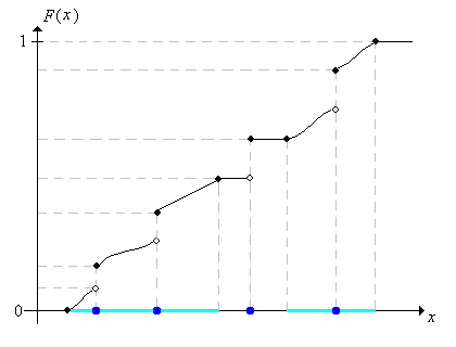
The distribution function is important because it makes sense for any type of random variable, regardless of whether the distribution is discrete, continuous, or even mixed, and because it completely determines the distribution of \(X\). In the picture below, the light shading is intended to represent a continuous distribution of probability, while the darker dots represents points of positive probability; \(F(x)\) is the total probability mass to the left of (and including) \(x\).

A few basic properties completely characterize distribution functions. Notationally, it will be helpful to abbreviate the limits of \(F\) from the left and right at \(x \in \R\), and at \(\infty\) and \(-\infty\) as follows: \[F(x^+) = \lim_{t \downarrow x} F(t), \; F(x^-) = \lim_{t \uparrow x} F(t), \; F(\infty) = \lim_{t \to \infty} F(t), \; F(-\infty) = \lim_{t \to -\infty} F(t) \]
Suppose that \( F \) is the distribution function of a real-valued random variable \( X \).
The proof relies on the increasing property of probability, relative to the subset partial order, and the continuity theorems.
The following result shows how the distribution function can be used to compute the probability that \(X\) is in an interval. Recall that a probability distribution on \((\R, \ms R)\) is completely determined by the probabilities of intervals; thus, the distribution function determines the distribution of \(X\).
Suppose again that \( F \) is the distribution function of a real-valued random variable \( X \). If \(a, \, b \in \R\) with \(a \lt b\) then
These results follow from definition , , and the difference rule: \(\P(B \setminus A) = \P(B) - \P(A) \) if \( A, \, B \) are events and \( A \subseteq B\).
Conversely, if a Function \(F: \R \to [0, 1]\) satisfies the basic properties in , then the formulas in define a probability distribution on \((\R, \ms R)\), with \(F\) as the distribution function. For more on this point, see the section on existence and uniqueness of positive measures.
If \(X\) has a continuous distribution, then the distribution function \(F\) is continuous.
Thus, the two meanings of continuous come together: continuous distribution and continuous function in the calculus sense. Next recall that the distribution of a real-valued random variable \( X \) is symmetric about a point \( a \in \R \) if the distribution of \( X - a \) is the same as the distribution of \( a - X \).
Suppose that \(X\) has a continuous distribution on \(\R\) that is symmetric about a point \(a\). Then the distribution function \(F\) satisfies \(F(a - t) = 1 - F(a + t)\) for \(t \in \R\).
Since \( X - a \) and \( a - X \) have the same distribution, \[ F(a - t) = \P(X \le a - t) = \P(X - a \le -t) = \P(a - X \le -t) = \P(X \ge a + t) = 1 - F(a + t) \]
There are simple relationships between the distribution function and the probability density function. Recall that if \(X\) takes value in \(S \in \ms R\) and has probability density function \(f\), we can extend \(f\) to all of \(\R\) by the convention that \(f(x) = 0\) for \(x \in S^c\). As in the definition in , it's customary to define the distribution function \(F\) on all of \(\R\), even if the random variable takes values in a subset.
Suppose that \(X\) has discrete distribution on a countable subset \(S \subseteq \R\). Let \(f\) denote the probability density function and \(F\) the distribution function.
Thus, \(F\) is a step function with jumps at the points in \(S\); the size of the jump at \(x\) is \(f(x)\).
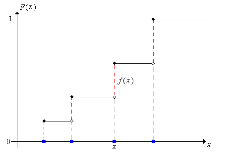
There is an analogous result for a continuous distribution with a probability density function.
Suppose that \(X\) has a continuous distribution on \(\R\) with distribution function \(F\) and with probability density function \(f\) that is piecewise continuous. Then
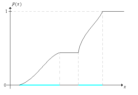
Proposition is the basic probabilistic version of the fundamental theorem of calculus. For mixed distributions, we have a combination of and propostion .
Suppose that \(X\) has a mixed distribution, with discrete part on a countable subset \(D \subseteq \R\), and continuous part on \(\R \setminus D\). Let \(g\) denote the partial probability density function of the discrete part and assume that the continuous part has partial probability density function \(h\) that is piecewise continuous. Let \(F\) denote the distribution function.
Go back to the graph of a general distribution function. At a point of positive probability, the probability is the size of the jump. At a smooth point of the graph, the continuous probability density is the slope.
Recall that a continuous distribution has a density function if and only if the distribution is absolutely continuous with respect to Lebesgue measure. But of course the distribution function always makes perfect sense. We have seen an example of a continuous distribution on the interval \((0, 1)\) that has no probability density function. The distribution function is continuous and strictly increases from 0 to 1 on the interval, but has derivative 0 at almost every point!
Naturally, the distribution function can be defined relative to any of the conditional distributions we have discussed. No new concepts are involved, and all of the results above hold.
Suppose again that \(X\) is a real-valued random variable with distribution function \(F\). The function in the following definition clearly gives the same information as \(F\).
The function \(F^c\) defined by \[ F^c(x) = 1 - F(x) = \P(X \gt x), \quad x \in \R\] is the right-tail distribution function of \(X\). Give the mathematical properties of \(F^c\) analogous to the properties in proposition of \(F\) in .
So \(F\) might be called the left-tail distribution function. But why have two distribution functions that give essentially the same information? The right-tail distribution function, and related functions, arise naturally in the context of reliability theory. For the remainder of this subsection, suppose that \(T\) is a random variable with values in \( [0, \infty) \) and that \( T \) has a continuous distribution with probability density function \( f \) that is piecewise continuous. We interpret \(T\) as the lifetime of a device, and we assume that \(F^c(t) \gt 0\) for \(t \in [0, \infty)\) so that the device can last for arbitrarily large periods of time. Here are the important defintions:
For the random lifetime \(T\),
To interpret the reliability function, note that \(F^c(t) = \P(T \gt t)\) is the probability that the device lasts at least \(t\) time units. To interpret the failure rate function, note that if \( dt \) is small
then
\[ \P(t \lt T \lt t + dt \mid T \gt t) = \frac{\P(t \lt T \lt t + dt)}{\P(T \gt t)} \approx \frac{f(t) \, dt}{F^c(t)} = h(t) \, dt \]
So \(h(t) \, dt\) is the approximate probability that the device will fail in the interval \((t, t + dt)\), given survival up to time \(t\). Moreover, like the distribution function and the reliability function, the failure rate function also completely determines the distribution of \(T\).
The reliability function can be expressed in terms of the failure rate function by \[ F^c(t) = \exp\left(-\int_0^t h(s) \, ds\right), \quad t \ge 0 \]
At the points of continuity of \( f \) we have \( \left[F^c\right]^\prime(t) = -f(t) \). Hence \[ \int_0^t h(s) \, ds = \int_0^t \frac{f(s)}{F^c(s)} \, ds = \int_0^t -\frac{\left[F^c\right]^\prime(s)}{F^c(s)} \, ds = -\ln\left[F^c(t)\right] \]
The failure rate function \(h\) satisfies the following properties:
Conversely, a function that satisfies these properties is the failure rate function for a continuous distribution on \( [0, \infty) \):
Suppose that \(h: [0, \infty) \to [0, \infty) \) is piecewise continuous and \(\int_0^\infty h(t) \, dt = \infty\). Then the function \( F^c \) defined by \[ F^c(t) = \exp\left(-\int_0^t h(s) \, ds\right), \quad t \ge 0 \] is a reliability function for a continuous distribution on \( [0, \infty) \)
The function \( F^c \) is continuous, decreasing, and satisfies \( F^c(0) = 1 \) and \( F^c(t) \to 0 \) as \( t \to \infty \). Hence \( F = 1 - F^c \) is the distribution function for a continuous distribution on \( [0, \infty) \).
Suppose now that \(X\) and \(Y\) are real-valued random variables for an experiment (that is, defined on the same probability space), so that \((X, Y)\) is random vector taking values in \(\R^2\).
The distribution function of \((X, Y)\) is the function \(F\) defined by \[ F(x, y) = \P(X \le x, Y \le y), \quad (x, y) \in \R^2\]
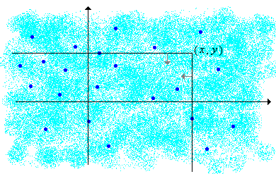
In the graph above, the light shading is intended to suggest a continuous distribution of probability, while the darker dots represent points of positive probability. Thus, \(F(x, y)\) is the total probability mass below and to the left (that is, southwest) of the point \((x, y)\). As in the single variable case, the distribution function of \((X, Y)\) completely determines the distribution of \((X, Y)\).
Suppose that \(a, \, b, \, c, \, d \in \R\) with \(a \lt b\) and \(c \lt d\). Then \[ \P(a \lt X \le b, c \lt Y \le d) = F(b, d) - F(a, d) - F(b, c) + F(a, c) \]
Note that \( \{X \le a, Y \le d\} \cup \{X \le b, Y \le c\} \cup \{a \lt X \le b, c \lt Y \le d\} = \{X \le b, Y \le d\} \). The intersection of the first two events is \( \{X \le a, Y \le c\} \) while the first and third events and the second and third events are disjoint. Thus, from the inclusion-exclusion rule we have \[ F(a, d) + F(b, c) + \P(a \lt X \le b, c \lt Y \le d) - F(a, c) = F(b, d) \]
A probability distribution on \( (\R^2, \ms R_2) \) is completely determined by its values on rectangles of the form \( (a, b] \times (c, d] \), so just as in the single variable case, it follows that the distribution function of \( (X, Y) \) completely determines the distribution of \( (X, Y) \).
In the setting of , give the appropriate formula on the right for all possible combinations of weak and strong inequalities on the left.
The joint distribution function determines the individual (marginal) distribution functions.
Let \(F\) denote the distribution function of \((X, Y)\), and let \(G\) and \(H\) denote the distribution functions of \(X\) and \(Y\), respectively. Then
These results follow from the continuity theorem for increasing events. For example, in (a) \[ \P(X \le x) = \P(X \le x, Y \lt \infty) = \lim_{y \to \infty} \P(X \le x, Y \le y) = \lim_{y \to \infty} F(x, y) \]
On the other hand, we cannot recover the distribution function of \( (X, Y) \) from the individual distribution functions, except when the variables are independent.
Random variables \(X\) and \(Y\) are independent if and only if \[ F(x, y) = G(x) H(y), \quad (x, y) \in \R^2\]
If \( X \) and \( Y \) are independent then \( F(x, y) = \P(X \le x, Y \le y) = \P(X \le x) \P(Y \le y) = G(x) H(y) \) for \( (x, y) \in \R^2 \). Conversely, suppose \( F(x, y) = G(x) H(y) \) for \( (x, y) \in \R^2 \). If \( a, \, b, \, c, \, d \in \R \) with \( a \lt b \) and \( c \lt d \) then from , \begin{align} \P(a \lt X \le b, c \lt Y \le d) & = G(b)H(d) - G(a)H(d) -G(b)H(c) + G(a)H(c) \\ & = [G(b) - G(a)][H(d) - H(c)] = \P(a \lt X \le b) \P(c \lt Y \le d) \end{align} so it follows that \( X \) and \( Y \) are independent. (Recall again that a probability distribution on \( (\R^2, \ms R_2) \) is completely determined by its values on rectangles.)
All of the results of this subsection generalize in a straightforward way to \(n\)-dimensional random vectors for \(n \in \N_+\). Only the notation is more complicated.
Suppose now that \( X \) is a real-valued random variable for a basic random experiment and that we repeat the experiment \( n \) times independently for some \(n \in \N_+\). This generates (for the new compound experiment) a sequence of independent variables \( (X_1, X_2, \ldots, X_n) \) each with the same distribution as \( X \). In statistical terms, this sequence is a random sample of size \( n \) from the distribution of \( X \). In statistical inference, the observed values \((x_1, x_2, \ldots, x_n)\) of the random sample form our data.
The empirical distribution function, based on the data \( (x_1, x_2, \ldots, x_n) \), is defined by \[ F_n(x) = \frac{1}{n} \#\left\{i \in \{1, 2, \ldots, n\}: x_i \le x\right\} = \frac{1}{n} \sum_{i=1}^n \bs{1}(x_i \le x), \quad x \in \R\]
Thus, \(F_n(x)\) gives the proportion of values in the data set that are less than or equal to \(x\). The function \(F_n\) is a statistical estimator of \(F\), based on the given data set. In addition, the empirical distribution function is related to the Brownian bridge.
Suppose again that \( X \) is a real-valued random variable with distribution function \( F \).
For \(p \in (0, 1)\), a value of \(x\) such that \( F(x^-) = \P(X \lt x) \le p\) and \(F(x) = \P(X \le x) \ge p\) is called a quantile of order \(p\) for the distribution.
Roughly speaking, a quantile of order \(p\) is a value where the graph of the distribution function crosses (or jumps over) \(p\). For example, in the picture below, \(a\) is the unique quantile of order \(p\) and \(b\) is the unique quantile of order \(q\). On the other hand, the quantiles of order \(r\) form the interval \([c, d]\), and moreover, \(d\) is a quantile for all orders in the interval \([r, s]\). Note also that if \( X \) has a continuous distribution (so that \( F \) is continuous) and \( x \) is a quantile of order \( p \in (0, 1) \), then \( F(x) = p \).
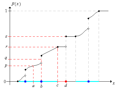
Note that there is an inverse relation of sorts between the quantiles and the cumulative distribution values, but the relation is more complicated than that of a function and its ordinary inverse function because the distribution function is not one-to-one in general. For many purposes, it is helpful to select a specific quantile for each order; to do this requires defining a generalized inverse of the distribution function \( F \).
The quantile function \( F^{-1} \) of \( X \) is defined by \[ F^{-1}(p) = \min\{x \in \R: F(x) \ge p\}, \quad p \in (0, 1)\]
\( F^{-1} \) is well defined: Since \(F\) is right continuous and increasing, \( \{x \in \R: F(x) \ge p\} \) is an interval of the form \( [a, \infty) \). Thus, the minimum of the set is \( a \).
Note that if \(F\) strictly increases from 0 to 1 on an interval \(S\) (so that the underlying distribution is continuous and is supported on \(S\)), then \(F^{-1}\) is the ordinary inverse of \(F\). We do not usually define the quantile function at the endpoints 0 and 1. If we did, note that \(F^{-1}(0)\) would always be \(-\infty\).
The following exercise justifies the name: \(F^{-1}(p)\) is the minimum of the quantiles of order \(p\).
Let \(p \in (0, 1)\).
Let \( y = F^{-1}(p) \).
Other basic properties of the quantile function are given in the following theorem.
\(F^{-1}\) satisfies the following properties:
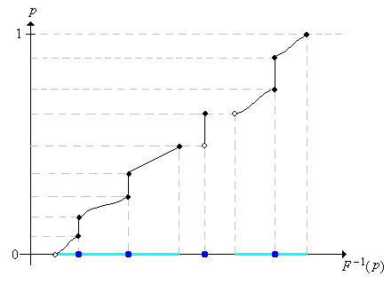
As always, the inverse of a function is obtained essentially by reversing the roles of independent and dependent variables. In the graphs below, note that jumps of \(F\) become flat portions of \(F^{-1}\) while flat portions of \(F\) become jumps of \(F^{-1}\). For \( p \in (0, 1) \), the set of quantiles of order \( p \) is the closed, bounded interval \( \left[F^{-1}(p), F^{-1}(p^+)\right] \). Thus, \( F^{-1}(p) \) is the smallest quantile of order \( p \), as we noted earlier, while \( F^{-1}(p^+) \) is the largest quantile of order \( p \).

The following basic property will be useful in simulating random variables.
For \(x \in \R\) and \(p \in (0, 1)\), \(F^{-1}(p) \le x\) if and only if \(p \le F(x)\).
Suppose that \( F^{-1}(p) \le x \). Then, since \( F \) is increasing, \( F\left[F^{-1}(p)\right] \le F(x) \). But \( p \le F\left[F^{-1}(p)\right] \) by part (c) of the previous result, so \( p \le F(x) \). Conversely, suppose that \( p \le F(x) \). Then, since \( F^{-1} \) is increasing, \( F^{-1}(p) \le F^{-1}[F(x)] \). But \( F^{-1}[F(x)] \le x \) by part (b) of the previous result, so \( F^{-1}(p) \le x \).
Certain quantiles are important enough to deserve special names.
Suppose that \( X \) is a real-valued random variable.
When there is only one median, it is frequently used as a measure of the center of the distribution, since it divides the set of values of \( X \) in half, by probability. More generally, the quartiles can be used to divide the set of values into fourths, by probability.
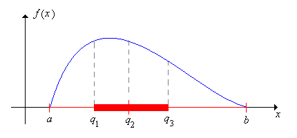
Assuming uniqueness, let \(q_1\), \(q_2\), and \(q_3\) denote the first, second, and third quartiles of \(X\), respectively, and let \(a = F^{-1}\left(0^+\right)\) and \(b = F^{-1}(1)\).
Note that the interval \( [q_1, q_3] \) roughly gives the middle half of the distribution, so the interquartile range, the length of the interval, is a natural measure of the dispersion of the distribution about the median. Note also that \(a\) and \(b\) are essentially the minimum and maximum values of \(X\), respectively, although of course, it's possible that \( a = -\infty \) or \( b = \infty \) (or both). Collectively, the five parameters give a great deal of information about the distribution in terms of the center, spread, and skewness. Graphically, the five numbers are often displayed as a boxplot or box and whisker plot, which consists of a line extending from the minimum value \(a\) to the maximum value \(b\), with a rectangular box from \(q_1\) to \(q_3\), and whiskers
at \(a\), the median \(q_2\), and \(b\). Roughly speaking, the five numbers separate the set of values of \(X\) into 4 intervals of approximate probability \(\frac{1}{4}\) each.
Suppose that \( X \) has a continuous distribution that is symmetric about a point \(a \in \R\). If \(a + t\) is a quantile of order \(p \in (0, 1) \) then \(a - t\) is a quantile of order \(1 - p\).
Note that this is the quantile function version of symmetry result in for the distribution function. If \( a + t \) is a qantile of order \( p \) then (since \( X \) has a continuous distribution) \( F(a + t) = p \). But then \( F(a - t) = 1 - F(a + t) = 1 - p \) so \( a - t \) is a quantile of order \( 1 - p \).
Let \(F\) be the function defined by \[ F(x) = \begin{cases} 0, & x \lt 1\\ \frac{1}{10}, & 1 \le x \lt \frac{3}{2}\\ \frac{3}{10}, & \frac{3}{2} \le x \lt 2\\ \frac{6}{10}, & 2 \le x \lt \frac{5}{2}\\ \frac{9}{10}, & \frac{5}{2} \le x \lt 3\\ 1, & x \ge 3; \end{cases}\]
Let \(F\) be the function defined by \[F(x) = \begin{cases} 0, & x \lt 0\\ \frac{x}{x + 1}, & x \ge 0 \end{cases}\]
The expression \( \frac{p}{1 - p} \) that occurs in the quantile function in the last exercise is known as the odds ratio associated with \( p \), particularly in the context of gambling. In statistics, it is sometimes referred to as relative risk.
Let \(F\) be the function defined by \[ F(x) = \begin{cases} 0, & x \lt 0\\ \frac{1}{4} x, & 0 \le x \lt 1\\ \frac{1}{3} + \frac{1}{4} (x - 1)^2, & 1 \le x \lt 2\\ \frac{2}{3} + \frac{1}{4} (x - 2)^3, & 2 \le x \lt 3\\ 1, & x \ge 3 \end{cases}\]
Suppose that \(X\) has probability density function \(f(x) = \frac{1}{b - a}\) for \(x \in [a, b]\), where \(a, \, b \in \R\) and \(a \lt b\).
The distribution in is the uniform distribution on the interval \( [a, b] \). The left endpoint \( a \) is the location parameter and the length of the interval \( w = b - a \) is the scale parameter. The uniform distribution models a point chose at random
from the interval.
In the quantile app, select the continuous uniform distribution. Vary the location and scale parameters and note the shape of the probability density function and the distribution function.
Suppose that \(T\) has probability density function \(f(t) = r e^{-r t}\) for \(t \in [0, \infty)\), where \(r \in (0, \infty)\) is a parameter.
The distribution in is the exponential distribution with rate parameter \(r\). Note that this distribution is characterized by the fact that it has constant failure rate (and this is the reason for referring to \( r \) as the rate parameter). The reciprocal of the rate parameter is the scale parameter. The exponential distribution is used to model failure times and other random times under certain conditions, particularly in the context of the Poisson model.
In the quantile app, select the exponential distribution. Vary the scale parameter \(b\) and note the shape of the probability density function and the distribution function.
Suppose that \(X\) has probability density function \(f(x) = \frac{a}{x^{a+1}}\) for \(x \in [1, \infty)\) where \(a \in (0, \infty)\) is a parameter.
The distribution in is the Pareto distribution with shape parameter \(a\), named after Vilfredo Pareto. The Pareto distribution is a heavy-tailed distribution that is sometimes used to model income and certain other economic variables.
In the quantile app, select the Pareto distribution. Keep the default value for the scale parameter, but vary the shape parameter and note the shape of the density function and the distribution function.
Suppose that \(X\) has probability density function \( f(x) = \frac{1}{\pi (1 + x^2)} \) for \(x \in \R\).
The distribution in is the Cauchy distribution, named after Augustin Cauchy.
In the quantile app, select the Cauchy distribution and keep the default parameter values. Note the shape of the density function and the distribution function.
Let \(h(t) = k t^{k - 1}\) for \(t \in (0, \infty)\) where \(k \in (0, \infty)\) is a parameter.
The distribution in is the Weibull distributions with shape parameter \(k\), named after Walodi Weibull. Since this family includes increasing, decreasing, and constant failure rates, it is widely used to model the lifetimes of various types of devices.
In the quantile app, select the Weibull distribution. Keep the default scale parameter, but vary the shape parameter and note the shape of the density function and the distribution function.
Suppose that \(X\) has probability density function \(f(x) = 12 x^2 (1 - x)\) for \(x \in [0, 1]\).
Suppose that \(X\) has probability density function \(f(x) = \frac{1}{\pi \sqrt{x (1 - x)}}\) for \(x \in (0, 1)\).
The distributions in and are examples of beta distributions. The particular beta distribution in is also known as the arcsine distribution; the distribution function explains the name.
In the quantile app, select the beta distribution. For each of the following parameter values, note the location and shape of the density function and the distribution function.
Let \(F(x) = \frac{e^x}{1 + e^x}\) for \(x \in \R\).
The distribution in is a logistic distribution and the quantile function is known as the logit function.
In the quantile app, select the logistic distribution and keep the default parameter values. Note the shape of the probability density function and the distribution function.
Let \(F(x) = e^{-e^{-x}}\) for \(x \in \R\).
The distribution in is the type 1 extreme value distribution, also known as the Gumbel distribution in honor of Emil Gumbel.
In the quantile app, select the extreme value distribution and keep the default parameter values. Note the shape and location of the probability density function and the distribution function.
Recall that the standard normal distribution has probability density function \( \phi \) given by \[ \phi(z) = \frac{1}{\sqrt{2 \pi}} e^{-\frac{1}{2} z^2}, \quad z \in \R\] This distribution models physical measurements of all sorts subject to small, random errors, and is one of the most important distributions in probability. The distribution function \( \Phi \), of course, can be expressed as \[ \Phi(z) = \int_{-\infty}^z \phi(x) \, dx, \quad z \in \R \] but \( \Phi \) and the quantile function \( \Phi^{-1} \) cannot be expressed, in closed from, in terms of elementary functions. Because of the importance of the normal distribution \( \Phi \) and \( \Phi^{-1} \) are themselves considered special functions, like \( \sin \), \( \ln \), and many others. Approximate values of these functions can be computed using most mathematical and statistical software packages. Because the distribution is symmetric about 0, \( \Phi(-z) = 1 - \Phi(z) \) for \( z \in \R \), and equivalently, \( \Phi^{-1}(1 - p) = -\Phi^{-1}(p)\). In particular, the median is 0.
Open the sepcial distribution calculator and choose the normal distribution. Keep the default parameter values and select CDF view. Note the shape and location of the distribution/quantile function. Compute each of the following:
Suppose that \(X\) has probability density function \(f(x) = -\ln x\) for \(x \in (0, 1)\).
Suppose that a pair of fair dice are rolled and the sequence of scores \((X_1, X_2)\) is recorded.
The random variables are discrete, so the CDFs are step functions, with jumps at the values of the variables. The following tables give the values of the CDFs at the values of the random variables.
| \(y\) | 2 | 3 | 4 | 5 | 6 | 7 | 8 | 9 | 10 | 11 | 12 |
|---|---|---|---|---|---|---|---|---|---|---|---|
| \(\P(Y \le y)\) | \(\frac{1}{36}\) | \(\frac{3}{36}\) | \(\frac{6}{36}\) | \(\frac{10}{36}\) | \(\frac{15}{36}\) | \(\frac{21}{36}\) | \(\frac{26}{36}\) | \(\frac{30}{36}\) | \(\frac{33}{36}\) | \(\frac{35}{36}\) | 1 |
| \(v\) | 1 | 2 | 3 | 4 | 5 | 6 |
|---|---|---|---|---|---|---|
| \(\P(V \le v)\) | \(\frac{1}{36}\) | \(\frac{4}{36}\) | \(\frac{9}{36}\) | \(\frac{16}{36}\) | \(\frac{25}{36}\) | 1 |
| \(y\) | 6 | 7 | 8 | 9 | 10 |
|---|---|---|---|---|---|
| \(\P(Y \le y \mid V = 5)\) | \(\frac{2}{9}\) | \(\frac{4}{9}\) | \(\frac{6}{9}\) | \(\frac{8}{9}\) | 1 |
Suppose that \((X, Y)\) has probability density function \(f(x, y) = x + y\) for \((x, y) \in [0, 1]^2\).
For the M&M data, compute the empirical distribution function of the total number of candies.
Let \(N\) denote the total number of candies. The empirical distribution function of \(N\) is a step function; the following table gives the values of the function at the jump points.
| \(n\) | 50 | 53 | 54 | 55 | 56 | 57 | 58 | 59 | 60 | 61 |
|---|---|---|---|---|---|---|---|---|---|---|
| \(\P(N \le n)\) | \(\frac{1}{30}\) | \(\frac{2}{30}\) | \(\frac{3}{30}\) | \(\frac{7}{30}\) | \(\frac{11}{30}\) | \(\frac{14}{30}\) | \(\frac{23}{30}\) | \(\frac{26}{30}\) | \(\frac{28}{30}\) | 1 |
For the cicada data, let \(BL\) denotes body length and let \(G\) denote gender. Compute the empirical distribution function of the following variables:
For statistical versions of some of the topics in this subsection, see the chapter on random samples, and in particular, the discussions of the sample mean and order statistics.