
The purpose of this section is to study how probabilities are updated in light of new information, clearly an absolutely essential topic. As usual, If you are a new student of probability, you may want to skip the measure-theoretic details.
As usual, we start with a ramdom experiment, modeled by a probability space \((S, \ms S, \P)\). So to review, \( S \) is the set of outcomes, \( \ms S \) the collection of events, and \( \P \) the probability measure on the sample space \( (S, \ms S) \). Suppose now that we know that an event \(B\) has occurred. In general, this information should clearly modfiy the probabilities that we should assign to other events. In particular, if \(A\) is another event then \(A\) occurs if and only if \(A\) and \(B\) occur; effectively, the sample space has been reduced to \(B\). Thus, the probability of \(A\), given that we know \(B\) has occurred, should be proportional to \(\P(A \cap B)\).
However, conditional probability, given that \(B\) has occurred, should still be a probability measure, that is, it must satisfy the axioms of probability. This forces the proportionality constant to be \(1 \big/ \P(B)\). Thus, we are led inexorably to the following definition:
Let \(A\) and \(B\) be events with \(\P(B) \gt 0\). The conditional probability of \(A\) given \(B\) is defined to be \[\P(A \mid B) = \frac{\P(A \cap B)}{\P(B)}\]
Definition is based on the axiomatic definition of probability. Let's explore the idea of conditional probability from the less formal and more intuitive notion of relative frequency (more precisely, the law of large numbers. Thus, suppose that we run the experiment repeatedly. For \( n \in \N_+ \) and an event \(E\), let \(N_n(E)\) denote the number of times \(E\) occurs (the frequency of \( E \)) in the first \(n\) runs. Note that \(N_n(E)\) is a random variable in the compound experiment that consists of replicating the original experiment. In particular, its value is unknown until we actually run the experiment \( n \) times.
Now, if \(N_n(B)\) is large, the conditional probability that \(A\) has occurred, given that \(B\) has occurred, should be close to the conditional relative frequency of \(A\) given \(B\), namely the relative frequency of \(A\) for the runs on which \(B\) occurred: \(N_n(A \cap B) / N_n(B)\). But note that \[\frac{N_n(A \cap B)}{N_n(B)} = \frac{N_n(A \cap B) / n}{N_n(B) / n}\] The numerator and denominator of the main fraction on the right are the relative frequencies of \( A \cap B \) and \( B \), respectively. So by the law of large numbers again, \( N_n(A \cap B) / n \to \P(A \cap B) \) as \( n \to \infty \) and \( N_n(B) \to \P(B) \) as \( n \to \infty \). Hence \[\frac{N_n(A \cap B)}{N_n(B)} \to \frac{\P(A \cap B)}{\P(B)} \text{ as } n \to \infty\] and we are led again to definition .
In some cases, conditional probabilities can be computed directly, by effectively reducing the sample space to the given event. In other cases, the formula in the mathematical definition is better. In some cases, conditional probabilities are known from modeling assumptions, and then are used to compute other probabilities. We will see examples of all of these cases in the computational exercises in below.
It's very important that you not confuse \(\P(A \mid B)\), the probability of \(A\) given \(B\), with \(\P(B \mid A)\), the probability of \(B\) given \(A\). Making that mistake is known as the fallacy of the transposed conditional. (How embarrassing!)
Suppose now that \((T, \ms T)\) is another measurable space, so that \(T\) is a set and \(\ms T\) is a \(\sigma\)-algebra of subsets of \(T\) (the measurable subsets of \(T\)). Recall that \(X\) is a random variable for the experiment with values in \(T\) if \( X \) is a measurable function from \( S \) into \( T \). This means that \( \{X \in A\} = \{s \in S: X(s) \in A\} \in \ms S \) for every \(A \in \ms T \). Intuitively, \( X \) is a variable of interest in the experiment, and every meaningful statement about \( X \) defines an event. Recall that the probability distribution of \(X\) is the probability measure on \( (T, \ms T) \) given by \[A \mapsto \P(X \in A), \quad A \in \ms T\] This has a natural extension to a conditional distribution, given an event.
If \(B\) is an event with \( \P(B) \gt 0 \), then the conditional distribution of \(X\) given \(B\) is the probability measure on \( (T, \ms T) \) given by \[A \mapsto \P(X \in A \mid B), \quad A \in \ms T\]
Our first result is of fundamental importance, and indeed was a crucial part of the argument for the definition of conditional probability.
Suppose again that \( B \) is an event with \( \P(B) \gt 0 \). Then \(A \mapsto \P(A \mid B)\) is a probability measure on \( (S, \ms S) \).
Clearly \( \P(A \mid B) \ge 0 \) for every event \( A \), and \( \P(S \mid B) = 1 \). Thus, suppose that \( \{A_i: i \in I\} \) is a countable collection of pairwise disjoint events. Then \[ \P\left(\bigcup_{i \in I} A_i \biggm| B\right) = \frac{1}{\P(B)} \P\left[\left(\bigcup_{i \in I} A_i\right) \cap B\right] = \frac{1}{\P(B)} \P\left(\bigcup_{i \in I} (A_i \cap B)\right) \] But the collection of events \( \{A_i \cap B: i \in I\} \) is also pairwise disjoint, so \[ \P\left(\bigcup_{i \in I} A_i \biggm| B\right) = \frac{1}{\P(B)} \sum_{i \in I} \P(A_i \cap B) = \sum_{i \in I} \frac{\P(A_i \cap B)}{\P(B)} = \sum_{i \in I} \P(A_i \mid B) \]
It's hard to overstate the importance of because this theorem means that any result that holds for probability measures in general holds for conditional probability, as long as the conditioning event remains fixed. In particular the basic probability rules have analogs for conditional probability. To give just two examples, suppose again that \(B\) is an event with \(\P(B) \gt 0\). \begin{align} \P\left(A^c \mid B\right) & = 1 - \P(A \mid B), \quad A \in \ms S \\ \P\left(A_1 \cup A_2 \mid B\right) & = \P\left(A_1 \mid B\right) + \P\left(A_2 \mid B\right) - \P\left(A_1 \cap A_2 \mid B\right), \quad A_1, \, A_2 \in \ms S \end{align} By the same token, it follows that the conditional distribution of a random variable with values in \( T \), given in , really does define a probability distribution on \( (T, \ms T) \). No further proof is necessary. Our next results are very simple.
Suppose that \(A\) and \(B\) are events with \( \P(B) \gt 0 \).
Parts (a) and (c) of certainly make sense. Suppose that we know that event \( B \) has occurred. If \( B \subseteq A \) then \( A \) becomes a certain event. If \( A \cap B = \emptyset \) then \( A \) becomes an impossible event. A conditional probability can be computed relative to a probability measure that is itself a conditional probability measure. The following result is a consitency condition.
Suppose that \(A\), \(B\), and \(C\) are events with \( \P(B \cap C) \gt 0 \). The probability of \(A\) given \(B\), relative to \(\P(\cdot \mid C)\), is the same as the probability of \(A\) given \(B\) and \(C\) (relative to \(\P\)). That is, \[\frac{\P(A \cap B \mid C)}{\P(B \mid C)} = \P(A \mid B \cap C)\]
Our next discussion concerns an important concept that deals with how two events are related, in a probabilistic sense.
Suppose that \(A\) and \(B\) are events with \( \P(A) \gt 0 \) and \( \P(B) \gt 0 \).
Intuitively, if \( A \) and \( B \) are positively correlated, then the occurrence of either event means that the other event is more likely. If \(A\) and \(B\) are negatively correlated, then the occurrence of either event means that the other event is less likely. If \(A\) and \(B\) are uncorrelated, then the occurrence of either event does not change the probability of the other event. Independence is a fundamental concept that can be extended to more than two events and to random variables. Correlation can also be generalized to random variables.
Suppose that \( A \) and \( B \) are events. Note from that if \( A \subseteq B \) or \( B \subseteq A \) then \( A \) and \( B \) are positively correlated. If \( A \) and \( B \) are disjoint then \( A \) and \( B \) are negatively correlated.
Suppose that \(A\) and \(B\) are events in a random experiment.
Sometimes conditional probabilities are known and can be used to find the probabilities of other events. Note first that if \( A \) and \( B \) are events with positive probability, then by definition , \[ \P(A \cap B) = \P(A) \P(B \mid A) = \P(B) \P(A \mid B) \] The following generalization is known as the multiplication rule of probability. As usual, we assume that any event conditioned on has positive probability.
Suppose that \(n \in \{2, 3, \ldots\}\) and that \((A_1, A_2, \ldots, A_n)\) is a sequence of events with \( \P(A_1 \cap A_2 \cap \cdots \cap A_{n-1}) \gt 0 \). Then \[\P\left(A_1 \cap A_2 \cap \cdots \cap A_n\right) = \P\left(A_1\right) \P\left(A_2 \mid A_1\right) P\left(A_3 \mid A_1 \cap A_2\right) \cdots \P\left(A_n \mid A_1 \cap A_2 \cap \cdots \cap A_{n-1}\right)\]
The product on the right a collapsing product in which only the probability of the intersection of all \(n\) events survives. The product of the first two factors is \( \P\left(A_1 \cap A_2\right) \), and hence the product of the first three factors is \( \P\left(A_1 \cap A_2 \cap A_3\right) \), and so forth. The proof can be made more rigorous by induction on \( n \).
The multiplication rule is particularly useful for experiments that consist of dependent stages, where \(A_i\) is an event in stage \(i\). Compare the multiplication rule of probability with the multiplication rule of combinatorics. As with any other result, the multiplication rule can be applied to a conditional probability measure.
In the context of , if \(E\) is another event, amd \( \P(A_1 \cap \cdots \cap A_{n-1} \cap E) \gt 0 \) then \[\P\left(A_1 \cap A_2 \cap \cdots \cap A_n \mid E\right) = \P\left(A_1 \mid E\right) \P\left(A_2 \mid A_1 \cap E\right) P\left(A_3 \mid A_1 \cap A_2 \cap E\right) \cdots \P\left(A_n \mid A_1 \cap A_2 \cap \cdots \cap A_{n-1} \cap E\right)\]
Suppose that \(\ms{A} = \{A_i: i \in I\}\) is a countable collection of events that partition the sample space \(S\) and that \( \P(A_i) \gt 0 \) for each \( i \in I \).

Theorem below is known as the law of total probability.
If \( B \) is an event then \[\P(B) = \sum_{i \in I} \P(A_i) \P(B \mid A_i)\]
Recall that \(\{A_i \cap B: i \in I\}\) is a partition of \(B\). Hence \[ \P(B) = \sum_{i \in I} \P(A_i \cap B) = \sum_{i \in I} \P(A_i) \P(B \mid A_i) \]
Theorem next is known as Bayes' Theorem, named after Thomas Bayes:
If \( B \) is an event then \[\P(A_j \mid B) = \frac{\P(A_j) \P(B \mid A_j)}{\sum_{i \in I}\P(A_i) \P(B \mid A_i)}, \quad j \in I\]
These two theorems are most useful, of course, when we know \(\P(A_i)\) and \(\P(B \mid A_i)\) for each \(i \in I\). When we compute the probability of \(\P(B)\) by the law of total probability , we say that we are conditioning on the partition \(\ms{A}\). Note that we can think of the sum as a weighted average of the conditional probabilities \(\P(B \mid A_i)\) over \(i \in I\), where \(\P(A_i)\), \(i \in I\) are the weight factors. In the context of Bayes' theorem , \(\P(A_j)\) is the prior probability of \(A_j\) and \(\P(A_j \mid B)\) is the posterior probability of \(A_j\) for \( j \in I \). We will study more general versions of conditioning and Bayes theorem for discrete distributioons and in terms of conditional expected value. Once again, the law of total probability and Bayes' theorem can be applied to a conditional probability measure.
If \(E\) is another event with \( \P(A_i \cap E) \gt 0 \) for \( i \in I \) then \begin{align} \P(B \mid E) & = \sum_{i \in I} \P(A_i \mid E) \P(B \mid A_i \cap E) \\ \P(A_j \mid B \cap E) & = \frac{\P(A_j \mid E) \P(B \mid A_j \cap E)}{\sum_{i \in I}\P(A_i \cap E) \P(B \mid A_i \cap E)}, \quad j \in I \end{align}
Suppose that \(A\) and \(B\) are events in an experiment with \(\P(A) = \frac{1}{3}\), \(\P(B) = \frac{1}{4}\), \(\P(A \cap B) = \frac{1}{10}\). Find each of the following:
Suppose that \(A\), \(B\), and \(C\) are events in a random experiment with \(\P(A \mid C) = \frac{1}{2}\), \(\P(B \mid C) = \frac{1}{3}\), and \(\P(A \cap B \mid C) = \frac{1}{4}\). Find each of the following:
Suppose that \(A\) and \(B\) are events in a random experiment with \(\P(A) = \frac{1}{2}\), \(\P(B) = \frac{1}{3}\), and \(\P(A \mid B) =\frac{3}{4}\).
Open the conditional probability experiment.
In a certain population, 30% of the persons smoke cigarettes and 8% have COPD (Chronic Obstructive Pulmonary Disease). Moreover, 12% of the persons who smoke have COPD.
A company has 200 employees: 120 are women and 80 are men. Of the 120 female employees, 30 are classified as managers, while 20 of the 80 male employees are managers. Suppose that an employee is chosen at random.
Consider the experiment that consists of rolling 2 standard, fair dice and recording the sequence of scores \(\bs{X} = (X_1, X_2)\). Let \(Y\) denote the sum of the scores. For each of the following pairs of events, find the probability of each event and the conditional probability of each event given the other. Determine whether the events are positively correlated, negatively correlated, or independent.
In each case below, the answers are for \( \P(A) \), \( \P(B) \), \( \P(A \mid B) \), and \( \P(B \mid A) \)
Note that positive correlation is not a transitive relation. From , for example, note that \(\{X_1 = 3\}\) and \(\{Y = 5\}\) are positively correlated, \(\{Y = 5\}\) and \(\{X_1 = 2\}\) are positively correlated, but \(\{X_1 = 3\}\) and \(\{X_1 = 2\}\) are negatively correlated (in fact, disjoint).
In dice experiment, set \(n = 2\). Run the experiment 1000 times. Compute the empirical conditional probabilities corresponding to the conditional probabilities in exercise .
Consider again the experiment that consists of rolling 2 standard, fair dice and recording the sequence of scores \(\bs{X} = (X_1, X_2)\). Let \(Y\) denote the sum of the scores, \(U\) the minimum score, and \(V\) the maximum score.
In the die-coin experiment, a standard, fair die is rolled and then a fair coin is tossed the number of times showing on the die. Let \(N\) denote the die score and \(H\) the event that all coin tosses result in heads.
Run the die-coin experiment 1000 times. Let \(H\) and \(N\) be as defined in exercise .
Suppose that a bag contains 12 coins: 5 are fair, 4 are biased with probability of heads \(\frac{1}{3}\); and 3 are two-headed. A coin is chosen at random from the bag and tossed.
Compare die-coin experiment in and the bag of coins experiment in . In the die-coin experiment, we toss a coin with a fixed probability of heads a random number of times. In the bag of coins experiment, we effectively toss a coin with a random probability of heads a fixed number of times. The random experiment of tossing a coin with a fixed probability of heads \(p\) a fixed number of times \(n\) is known as the binomial experiment with parameters \(n\) and \(p\). So the die-coin and bag of coins experiments can be thought of as modifications of the binomial experiment in which a parameter has been randomized. In general, interesting new random experiments can often be constructed by randomizing one or more parameters in another random experiment.
In the coin-die experiment, a fair coin is tossed. If the coin lands tails, a fair die is rolled. If the coin lands heads, an ace-six flat die is tossed (faces 1 and 6 have probability \(\frac{1}{4}\) each, while faces 2, 3, 4, and 5 have probability \(\frac{1}{8}\) each). Let \(H\) denote the event that the coin lands heads, and let \(Y\) denote the score when the chosen die is tossed.
Run the coin-die experiment 1000 times. Let \(H\) and \(Y\) be as defined in .
Consider the card experiment that consists of dealing 2 cards from a standard deck and recording the sequence of cards dealt. For \(i \in \{1, 2\}\), let \(Q_i\) be the event that card \(i\) is a queen and \(H_i\) the event that card \(i\) is a heart. For each of the following pairs of events, compute the probability of each event, and the conditional probability of each event given the other. Determine whether the events are positively correlated, negatively correlated, or independent.
The answers below are for \( \P(A) \), \( \P(B) \), \( \P(A \mid B) \), and \( \P(B \mid A) \) where \( A \) and \( B \) are the given events
In the card experiment, set \(n = 2\). Run the experiment 500 times. Compute the conditional relative frequencies corresponding to the conditional probabilities in exercise .
Consider the card experiment that consists of dealing 3 cards from a standard deck and recording the sequence of cards dealt. Find the probability of the following events:
In the card experiment, set \(n = 3\) and run the simulation 1000 times. Compute the empirical probability of each event in exercise and compare with the true probability.
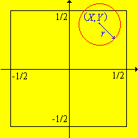
Recall that Buffon's coin experiment consists of tossing a coin with radius \(r \le \frac{1}{2}\) randomly on a floor covered with square tiles of side length 1. The coordinates \((X, Y)\) of the center of the coin are recorded relative to axes through the center of the square, parallel to the sides. Since the needle is dropped randomly, the basic modeling assumption is that \( (X, Y) \) is uniformly distributed on the square \( [-1/2, 1/2]^2 \).
In Buffon's coin experiment,
Run Buffon's coin experiment 500 times. Compute the empirical probability that \(Y \gt 0\) given that \(X \lt Y\) and compare with the probability in exercise .
In the conditional probability experiment, the random points are uniformly distributed on the rectangle \( S \). Move and resize events \( A \) and \( B \) and note how the probabilities change. For each of the following configurations, run the experiment 1000 times and compare the relative frequencies with the true probabilities.
A plant has 3 assembly lines that produces memory chips. Line 1 produces 50% of the chips and has a defective rate of 4%; line 2 has produces 30% of the chips and has a defective rate of 5%; line 3 produces 20% of the chips and has a defective rate of 1%. A chip is chosen at random from the plant.
Suppose that a bit (0 or 1) is sent through a noisy communications channel. Because of the noise, the bit sent may be received incorrectly as the complementary bit. Specifically, suppose that if 0 is sent, then the probability that 0 is received is 0.9 and the probability that 1 is received is 0.1. If 1 is sent, then the probability that 1 is received is 0.8 and the probability that 0 is received is 0.2. Finally, suppose that 1 is sent with probability 0.6 and 0 is sent with probability 0.4. Find the probability that
Suppose that \(T\) denotes the lifetime of a light bulb (in 1000 hour units), and that \(T\) has the following exponential distribution, defined for measurable \(A \subseteq [0, \infty)\): \[\P(T \in A) = \int_A e^{-t} dt\]
Suppose again that \(T\) denotes the lifetime of a light bulb (in 1000 hour units), but that \(T\) is uniformly distributed on the interal \([0, 10]\).
Refer to the previus discussion of genetics if you need to review some of the definitions in this section. Recall first that the ABO blood type in humans is determined by three alleles: \(a\), \(b\), and \(o\). Furthermore, \(a\) and \(b\) are co-dominant and \(o\) is recessive. Suppose that the probability distribution for the set of blood genotypes in a certain population is given in the following table:
| Genotype | \(aa\) | \(ab\) | \(ao\) | \(bb\) | \(bo\) | \(oo\) |
|---|---|---|---|---|---|---|
| Probability | 0.050 | 0.038 | 0.310 | 0.007 | 0.116 | 0.479 |
Suppose that a person is chosen at random from the population. Let \(A\), \(B\), \(AB\), and \(O\) be the events that the person is type \(A\), type \(B\), type \(AB\), and type \(O\) respectively. Let \(H\) be the event that the person is homozygous, and let \(D\) denote the event that the person has an \(o\) allele. Find each of the following:
Suppose next that pod color in certain type of pea plant is determined by a gene with two alleles: \(g\) for green and \(y\) for yellow, and that \(g\) is dominant and \(y\) recessive.
Suppose that a green-pod plant and a yellow-pod plant are bred together. Suppose further that the green-pod plant has a \(\frac{1}{4}\) chance of carrying the recessive yellow-pod allele.
Suppose that two green-pod plants are bred together. Suppose further that with probability \(\frac{1}{3}\) neither plant has the recessive allele, with probability \(\frac{1}{2}\) one plant has the recessive allele, and with probability \(\frac{1}{6}\) both plants have the recessive allele.
Next consider a sex-linked hereditary disorder in humans (such as colorblindness or hemophilia). Let \(h\) denote the healthy allele and \(d\) the defective allele for the gene linked to the disorder. Recall that \(h\) is dominant and \(d\) recessive for women.
Suppose that in a certain population, 50% are male and 50% are female. Moreover, suppose that 10% of males are color blind but only 1% of females are color blind.
Since color blindness is a sex-linked hereditary disorder, note that it's reasonable in exercise that the probability that a female is color blind is the square of the probability that a male is color blind. If \(p\) is the probability of the defective allele on the \(X\) chromosome, then \(p\) is also the probability that a male will be color blind. But since the defective allele is recessive, a woman would need two copies of the defective allele to be color blind, and assuming independence, the probability of this event is \(p^2\).
A man and a woman do not have a certain sex-linked hereditary disorder, but the woman has a \(\frac{1}{3}\) chance of being a carrier.
Urn 1 contains 4 red and 6 green balls while urn 2 contains 7 red and 3 green balls. An urn is chosen at random and then a ball is chosen at random from the selected urn.
Urn 1 contains 4 red and 6 green balls while urn 2 contains 6 red and 3 green balls. A ball is selected at random from urn 1 and transferred to urn 2. Then a ball is selected at random from urn 2.
An urn initially contains 6 red and 4 green balls. A ball is chosen at random from the urn and its color is recorded. It is then replaced in the urn and 2 new balls of the same color are added to the urn. The process is repeated. Find the probability of each of the following events:
Think about the results in exercise . Note in particular that the answers to parts (a), (b), and (c) are the same, and that the probability that the second ball is red in part (d) is the same as the probability that the first ball is red. More generally, the probabilities of events do not depend on the order of the draws. For example, the probability of an event involving the first, second, and third draws is the same as the probability of the corresponding event involving the seventh, tenth and fifth draws. Technically, the sequence of events \((R_1, R_2, \ldots)\) is exchangeable. The random process described in this exercise is a special case of Pólya's urn scheme, named after George Pólya.
An urn initially contains 6 red and 4 green balls. A ball is chosen at random from the urn and its color is recorded. It is then replaced in the urn and two new balls of the other color are added to the urn. The process is repeated. Find the probability of each of the following events:
Think about the results in , and compare with Pólya's urn . Note that the answers to parts (a), (b), and (c) are not all the same, and that the probability that the second ball is red in part (d) is not the same as the probability that the first ball is red. In short, the sequence of events \((R_1, R_2, \ldots)\) is not exchangeable.
Suppose that we have a random experiment with an event \(A\) of interest. When we run the experiment, of course, event \(A\) will either occur or not occur. However, suppose that we are not able to observe the occurrence or non-occurrence of \(A\) directly. Instead we have a diagnostic test designed to indicate the occurrence of event \(A\); thus the test that can be either positive for \(A\) or negative for \(A\). The test also has an element of randomness, and in particular can be in error.
Typical examples of events of interest and corresponding diagnostic tests:
Here are the critical defnitions:
Let \(T\) be the event that the test is positive for the occurrence of \(A\).
In many cases, the sensitivity and specificity of the test are known, as a result of the development of the test. However, the user of the test is interested in the opposite conditional probabilities, namely \(\P(A \mid T)\), the probability of the event of interest, given a positive test, and \(\P(A^c \mid T^c)\), the probability of the complementary event, given a negative test. Of course, if we know \( \P(A \mid T) \) then we also have \( \P(A^c \mid T) = 1 - \P(A \mid T) \), the probability of the complementary event given a positive test. Similarly, if we know \( \P(A^c \mid T^c) \) then we also have \( \P(A \mid T^c) \), the probability of the event given a negative test. Computing the probabilities of interest is simply a special case of Bayes' theorem .
The probability that the event occurs, given a positive test is \[\P(A \mid T) = \frac{\P(A) \P(T \mid A)}{\P(A) \P(T \mid A) + \P(A^c) \P(T \mid A^c)}\] The probability that the event does not occur, given a negative test is \[\P(A^c \mid T^c) = \frac{\P(A^c) \P(T^c \mid A^c)}{\P(A) \P(T^c \mid A) + \P(A^c) \P(T^c \mid A^c)}\]
There is often a tradeoff between sensitivity and specificity. An attempt to make a test more sensitive may result in the test being less specific, and an attempt to make a test more specific may result in the test being less sensitive. As an extreme example, consider the worthless test that always returns positive, no matter what the evidence. Then \( T = S \), the set of all outcomes, so the test has sensitivity 1, but specificity 0. At the opposite extreme is the worthless test that always returns negative, no matter what the evidence. Then \( T = \emptyset \) so the test has specificity 1 but sensitivity 0. In between these extremes are helpful tests that are actually based on evidence of some sort.
Suppose that the sensitivity \( a = \P(T \mid A) \in (0, 1)\) and the specificity \( b = \P(T^c \mid A^c) \in (0, 1) \) are fixed. Let \( p = \P(A) \) denote the prior probability of the event \( A \) and \( P = \P(A \mid T) \) the posterior probability of \( A \) given a positive test.
\( P \) as a function of \( p \) is given by \[ P = \frac{a p}{(a + b - 1) p + (1 - b)}, \quad p \in [0, 1] \]
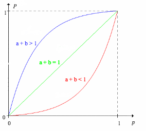
The formula for \( P \) in terms of \( p \) follows from the conditional probabilities in above and algebra. For part (a), note that \[ \frac{dP}{dp} = \frac{a (1 - b)}{[(a + b - 1) p + (1 - b)]^2} \gt 0\] For parts (b)–(d), note that \[ \frac{d^2 P}{dp^2} = \frac{-2 a (1 - b)(a + b - 1)}{[(1 + b - 1)p + (1 - b)]^3} \] If \( a + b \gt 1 \), \( d^2P/dp^2 \lt 0 \) so \( P \) is concave downward on \( [0, 1] \) and hence \( P \gt p \) for \( 0 \lt p \lt 1 \). If \( a + b \lt 1 \), \( d^2P/dp^2 \gt 0 \) so \( P \) is concave upward on \( [0, 1] \) and hence \( P \lt p \) for \( 0 \lt p \lt 1 \). Trivially if \( a + b = 1 \), \( P = p \) for \( 0 \le p \le 1 \).
Of course, part (b) of is the typical case, where the test is useful. In fact, we would hope that the sensitivity and specificity are close to 1. In case (c), the test is worse than useless since it gives the wrong information about \( A \). But this case could be turned into a useful test by simply reversing the roles of positive and negative. In case (d), the test is worthless and gives no information about \( A \). It's interesting that the broad classification above depends only on the sum of the sensitivity and specificity.
Suppose that a diagnostic test has sensitivity 0.99 and specificity 0.95. Find \( \P(A \mid T) \) for each of the following values of \( \P(A) \):
With sensitivity 0.99 and specificity 0.95, the test in the last exercise superficially looks good. However the small value of \(\P(A \mid T)\) for small values of \(\P(A)\) is striking (but inevitable given the properties in ). The moral, of course, is that \(\P(A \mid T)\) depends critically on \(\P(A)\) not just on the sensitivity and specificity of the test. Moreover, the correct comparison is \(\P(A \mid T)\) with \(\P(A)\), as in the exercise, not \(\P(A \mid T)\) with \(\P(T \mid A)\)—Beware of the fallacy of the transposed conditional! In terms of the correct comparison, the test does indeed work well; \(\P(A \mid T)\) is significantly larger than \(\P(A)\) in all cases.
A woman initially believes that there is an even chance that she is or is not pregnant. She takes a home pregnancy test with sensitivity 0.95 and specificity 0.90 (which are reasonable values for a home pregnancy test). Find the updated probability that the woman is pregnant in each of the following cases.
Suppose that 70% of defendants brought to trial for a certain type of crime are guilty. Moreover, historical data show that juries convict guilty persons 80% of the time and convict innocent persons 10% of the time. Suppose that a person is tried for a crime of this type. Find the updated probability that the person is guilty in each of the following cases:
The Check Engine
light on your car has turned on. Without the information from the light, you believe that there is a 10% chance that your car has a serious engine problem. You learn that if the car has such a problem, the light will come on with probability 0.99, but if the car does not have a serious problem, the light will still come on, under circumstances similar to yours, with probability 0.3. Find the updated probability that you have an engine problem.
0.268
The standard test for HIV is the ELISA (Enzyme-Linked Immunosorbent Assay) test. It has sensitivity and specificity of 0.999. Suppose that a person is selected at random from a population in which 1% are infected with HIV, and given the ELISA test. Find the probability that the person has HIV in each of the following cases:
The ELISA test for HIV is a very good one. Let's look another test, this one for prostate cancer, that's rather bad.
The PSA test for prostate cancer is based on a blood marker known as the Prostate Specific Antigen. An elevated level of PSA is evidence for prostate cancer. To have a diagnostic test, in the sense that we are discussing here, we must decide on a definite level of PSA, above which we declare the test to be positive. A positive test would typically lead to other more invasive tests (such as biopsy) which, of course, carry risks and cost. The PSA test with cutoff 2.6 ng/ml has sensitivity 0.40 and specificity 0.81. The overall incidence of prostate cancer among males is 156 per 100000. Suppose that a man, with no particular risk factors, has the PSA test. Find the probability that the man has prostate cancer in each of the following cases:
In fairness, the PSA test is medically useful if taken regularly. A sudden increase in PSA is a good predictor of prostate cancer.
The rapid molecular test for COVID-19 has sensitivity 0.952 and specificity of 0.0.980. Suppose that a person is selected at random from a population in which 10% are infected with COVID-19, and given the rapid test. Find the probability that the person is infected with COVID-19 in each of the following cases:
Diagnostic testing is closely related to a general statistical procedure known as hypothesis testing.
For the M&M data set, find the empirical probability that a bag has at least 10 reds, given that the weight of the bag is at least 48 grams.
\(\frac{10}{23}\).
Consider the Cicada data.