Buffon's experiments are very old and famous random experiments, named after comte de Buffon. These experiments are considered to be among the first problems in geometric probability.
Buffon's coin experiment consists of dropping a coin randomly on a floor covered with identically shaped tiles. The event of interest is that the coin crosses a crack between tiles. We will model Buffon's coin problem with square tiles of side length 1—assuming the side length is 1 is equivalent to taking the side length as the unit of measurement.
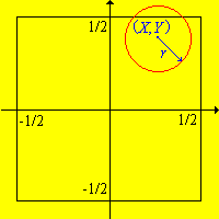
First, let us define the experiment mathematically. As usual, we will idealize the physical objects by assuming that the coin is a perfect circle with radius \(r\) and that the cracks between tiles are line segments. A natural way to describe the outcome of the experiment is to record the center of the coin relative to the center of the tile where the coin happens to fall. More precisely, we will construct coordinate axes so that the tile where the coin falls occupies the square \( S = \left[ -\frac{1}{2}, \frac{1}{2} \right]^2 \).
Now when the coin is tossed, we will denote the center of the coin by \((X, Y) \in S\). So the sample space is \((S, \ms S)\) where \(\ms S\) is the standard collectiion of subsets of \(S\), and \(X\) and \(Y\) are our basic random variables. Finally, we will assume that \(r \lt \frac{1}{2}\) so that it is at least possible for the coin to fall inside the square without touching a crack.

Next, we need to define an appropriate probability measure that describes our basic random vector \((X, Y)\). If the coin falls randomly
on the floor, then it is natural to assume that \((X, Y)\) is uniformly distributed on \(S\). By definition, this means that
Run Buffon's coin experiment with the default settings. Watch how the points seem to fill the sample space \(S\) in a uniform manner.
Our interest is in the probability of the event \(C\) that the coin crosses a crack.
The probability of a crack crossing is \(\P(C) - 1 - (1 - 2 r)^2\).
Note that in terms of the basic variables, \(C^c = \left\{r - \frac{1}{2} \lt X \lt \frac{1}{2} - r, r - \frac{1}{2} \lt Y \lt \frac{1}{2} - r\right\}\).
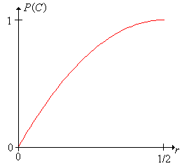
In Buffon's coin experiment, change the radius with the scrollbar and watch how the events \(C\) and \(C^c\) and change. Run the experiment with various values of \(r\) and compare the physical experiment with the points in the scatterplot. Compare the relative frequency of \(C\) to the probability of \(C\).
The convergence of the relative frequency of an event (as the experiment is repeated) to the probability of the event is a special case of the law of large numbers.
Solve Buffon's coin problem with rectangular tiles that have height \(h\) and width \(w\).
\[1 - \frac{(h - 2 \, r)(w - 2 \, r)}{h \, w}, \quad r \lt \min \left\{ \frac{h}{2}, \frac{w}{2} \right\}\]
Solve Buffon's coin problem with equilateral triangular tiles that have side length 1.
Recall that random numbers are simulation of independent random variables, each with the standard uniform distribution, that is, the continuous uniform distribution on the interval \( (0, 1) \).
Show how to simulate the center of the coin \((X, Y)\) in Buffon's coin experiment using random numbers.
\(X = U - \frac{1}{2}\), \(Y = V - \frac{1}{2}\), where \(U\) and \(V\) are random numbers.
Buffon's needle experiment consists of dropping a needle on a hardwood floor. The main event of interest is that the needle crosses a crack between floorboards. Strangely enough, the probability of this event leads to a statistical estimate of the number \(\pi\)!
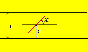
Our first step is to define the experiment mathematically. Again we idealize the physical objects by assuming that the floorboards are uniform and that each has width 1. We will also assume that the needle has length \(L \lt 1\) so that the needle cannot cross more than one crack. Finally, we assume that the cracks between the floorboards and the needle are line segments.
When the needle is dropped, we want to record its orientation relative to the floorboard cracks. One way to do this is to record the angle \(X\) that the top half of the needle makes with the line through the center of the needle, parallel to the floorboards, and the distance \(Y\) from the center of the needle to the bottom crack. These will be the basic random variables of our experiment, and thus the sample space of the experiment is \((S, \ms S)\) where \(S = [0, \pi) \times [0, 1)\) and where \(\ms S\) is the standard collection of subsets of \(S\).
Again, our main modeling assumption is that the needle is tossed randomly
on the floor. Thus, a reasonable mathematical assumption might be that the basic random vector \((X, Y)\) is uniformly distributed over the sample space. By definition, this means that
\[ \P[(X, Y) \in A] = \frac{\area(A)}{\area(S)}, \quad A \in \ms S \]
Run Buffon's needle experiment with the default settings and watch the outcomes being plotted in the sample space. Note how the points in the scatterplot seem to fill the sample space \(S\) in a uniform way.
Our main interest is in the event \(C\) that the needle crosses a crack between the floorboards.
The event \(C\) can be written in terms of the basic angle and distance variables as follows: \[ C = \left\{ Y \lt \frac{L}{2} \, \sin(X) \right\} \cup \left\{ Y \gt 1 - \frac{L}{2} \, \sin(X) \right\} \]
The curves \(y = \frac{L}{2} \, \sin(x)\) and \(y = 1 - \frac{L}{2} \, \sin(x)\) on the interval \(0 \le x \lt \pi\) are shown in blue in the scatterplot of Buffon's needle experiment, and hence event \(C\) is the union of the regions below the lower curve and above the upper curve. Thus, the needle crosses a crack precisely when a point falls in this region.
The probability of a crack crossing is \(\P(C) = 2 L / \pi\).
From symmetry and simple calculus it follows that \(\area(C) = 2 L\). Of course \(\area(S) = \pi\).
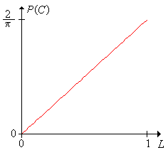
In the Buffon's needle experiment, vary the needle length \(L\) with the scrollbar and watch how the event \(C\) changes. Run the experiment with various values of \(L\) and compare the physical experiment with the points in the scatterplot. Compare the relative frequency of \(C\) to the probability of \(C\).
The convergence of the relative frequency of an event (as the experiment is repeated) to the probability of the event is a special case of the law of large numbers.
Find the probabilities of the following events in Buffon's needle experiment. In each case, sketch the event as a subset of the sample space.
Suppose that we run Buffon's needle experiment a large number of times. By the law of large numbers, the proportion of crack crossings should be about the same as the probability of a crack crossing. More precisely, we will denote the number of crack crossings in the first \(n\) runs by \(N_n\). Note that \(N_n\) is a random variable for the compound experiment that consists of \(n\) replications of the basic needle experiment. Thus, if \(n\) is large, we should have \( \frac{N_n}{n} \approx \frac{2 L}{\pi} \) and hence \[ \pi \approx \frac{2 L n}{N_n} \] This is Buffon's famous estimate of \(\pi\).
Run the Buffon's needle experiment with needle lengths \(L \in \{0.3, 0.5, 0.7, 1\}\). In each case, watch the estimate of \(\pi\) as the simulation runs.
Let us analyze the estimation problem more carefully. On each run \(j\) we have an indicator variable \(I_j\), where \(I_j = 1\) if the needle crosses a crack on run \(j\) and \(I_j = 0\) if the needle does not cross a crack on run \(j\). These indicator variables are independent, and identically distributed, since we are assuming independent replications of the experiment. Thus, the sequence forms a Bernoulli trials process.
The number of crack crossings in the first \(n\) runs of the experiment is \[ N_n = \sum_{j=1}^n I_j \] which has the binomial distribution with parameters \(n\) and \(2 L / \pi\).
The mean and variance of \(N_n\) are
With probability 1, \(\frac{N_n}{2 L n} \to \frac{1}{\pi}\) as \(n \to \infty\) and \(\frac{2 L n}{N_n} \to \pi\) as \(n \to \infty\).
These results follow from the strong law of large numbers.
So we have two basic estimators: \(\frac{N_n}{2 L n}\) as an estimator of \(\frac{1}{\pi}\) and \(\frac{2 L n}{N_n}\) as an estimator of \(\pi\). The estimator of \(\frac{1}{\pi}\) has several important statistical properties. First, it is unbiased since the expected value of the estimator is the parameter being estimated:
The estimator of \(\frac{1}{\pi}\) is unbiased: \[ \E \left( \frac{N_n}{2 L n} \right) = \frac{1}{\pi} \]
This follows from the results above for the binomial distribution in and properties of expected value.
Since this estimator is unbiased, the variance gives the mean square error: \[ \var \left( \frac{N_n}{2 L n} \right) = \E \left[ \left( \frac{N_n}{2 L n} - \frac{1}{\pi} \right)^2 \right] \]
The mean square error of the estimator of \( \frac{1}{\pi} \) is \[ \var \left( \frac{N_n}{2 L n} \right) = \frac{\pi - 2 L}{2 L n \pi^2} \]
The variance is a decreasing function of the needle length \(L\).
So the estimator of \(\frac{1}{\pi}\) improves as the needle length increases. On the other hand, the estimator of \(\pi\) is biased; it tends to overestimate \(\pi\):
The estimator of \(\pi\) is positively biased: \[ \E \left( \frac{2 L n}{N_n} \right) \ge \pi \]
This follows from Jensen's inequality.
The estimator of \(\pi\) also tends to improve as the needle length increases. This is not easy to see mathematically. However, you can see it empirically.
In the Buffon's needle experiment, run the simulation 5000 times each with \(L = 0.3\), \(L = 0.5\), \(L = 0.7\), and \(L = 0.9\). Note how well the estimator seems to work in each case.
Finally, we should note that as a practical matter, Buffon's needle experiment is not a very efficient method of approximating \(\pi\). To estimate \(\pi\) to four decimal places with \(L = \frac{1}{2}\) would require about 100 million tosses!
Run the Buffon's needle experiment until the estimates of \(\pi\) seem to be consistently correct to two decimal places. Note the number of runs required. Try this for needle lengths \(L = 0.3\), \(L = 0.5\), \(L = 0.7\), and \(L = 0.9\) and compare the results.
Show how to simulate the angle \(X\) and distance \(Y\) in Buffon's needle experiment using random numbers.
\(X = \pi U\), \(Y = V\), where \(U\) and \(V\) are random numbers.
Buffon's needle problem is essentially solved by Monte-Carlo integration. In general, Monte-Carlo methods use statistical sampling to approximate the solutions of problems that are difficult to solve analytically. The modern theory of Monte-Carlo methods began with Stanislaw Ulam, who used the methods on problems associated with the development of the hydrogen bomb.
The original needle problem has been extended in many ways, starting with Simon Laplace who considered a floor with rectangular tiles. Indeed, variations on the problem are active research problems even today.
Neil Weiss has pointed out that our computer simulation of Buffon's needle experiment is circular, in the sense the program assumes knowledge of \(\pi\) (you can see this from ).
Try to write a computer algorithm for Buffon's needle problem, without assuming the value of \(\pi\) or any other transcendental numbers.