In a queuing model, customers arrive at a station for service. As always, the terms are generic; here are some typical examples:

Queuing models can be quite complex, depending on such factors as the probability distribution that governs the arrival of customers, the probability distribution that governs the service of customers, the number of servers, and the behavior of the customers when all servers are busy. Indeed, queuing theory has its own lexicon to indicate some of these factors. In this section, we will study one of the simplest, discrete-time queuing models. However, as we will see, this discrete-time chain is embedded in a much more realistic continuous-time queuing process knows as the M/G/1 queue. In a general sense, the main interest in any queuing model is the number of customers in the system as a function of time, and in particular, whether the servers can adequately handle the flow of customers.
Our main assumptions are as follows:
Thus, let \( X_n \) denote the number of customers in the system at time \( n \in \N \), and let \( U_n \) denote the number of new customers who arrive at time \( n \in \N_+ \). Then \( \bs{U} = (U_1, U_2, \ldots) \) is a sequence of independent random variables, with common probability density function \( f \) on \( \N \), and \[ X_{n+1} = \begin{cases} U_{n+1}, & X_n = 0 \\ (X_n - 1) + U_{n+1}, & X_n \gt 0 \end{cases}, \quad n \in \N \]
\( \bs{X} = (X_0, X_1, X_2, \ldots) \) is a discrete-time Markov chain with state space \( \N \) and transition probability matrix \( P \) given by \begin{align} P(0, y) & = f(y), \quad y \in \N \\ P(x, y) & = f(y - x + 1), \quad x \in \N_+, \; y \in \{x - 1, x, x + 1, \ldots\} \end{align} The chain \( \bs{X} \) is the queuing chain with arrival distribution defined by \( f \).
The Markov property and the form of the transition matrix follow from the construction of the state process \( \bs{X} \) in term of the IID sequence \( \bs{U} \). Starting in state 0 (an empty queue), a random number of new customers arrive at the next time unit, governed by the PDF \( f \). Hence the probability of going from state 0 to state \( y \) in one step is \( f(y) \). Starting in state \( x \in \N_+ \), one customer is served and a random number of new customers arrive by the next time unit, again governed by the PDF \( f \). Hence the probability of going from state \( x \) to state \( y \in \{x - 1, x, x + 1, \ldots\} \) is \( f[y - (x - 1)] \).
From now on we will assume that \( f(0) \gt 0 \) and \( f(0) + f(1) \lt 1 \). Thus, at each time unit, it's possible that no new customers arrive or that at least 2 new customers arrive. Also, we let \( m \) denote the mean of the arrival distribution, so that \[ m = \sum_{x = 0}^\infty x f(x) \] Thus \( m \) is the average number of new customers who arrive during a time period.
The chain \( \bs{X} \) is irreducible and aperiodic.
In a positive state, the chain can move at least one unit to the right and can move one unit to the left at the next step. From state 0, the chain can move two or more units to the right or can stay in 0 at the next step. Thus, every state leads to every other state so the chain is irreducible. Since 0 leads back to 0, the chain is aperiodic.
Our goal in this section is to compute the probability that the chain reaches 0, as a function of the initial state (so that the server is able to serve all of the customers). As we will see, there are some curious and unexpected parallels between this problem and the problem of computing the extinction probability in the branching chain. As a corollary, we will also be able to classify the queuing chain as transient or recurrent. Our basic parameter of interest is \( q = H(1, 0) = \P(\tau_0 \lt \infty \mid X_0 = 1) \), where as usual, \( H \) is the hitting probability matrix and \( \tau_0 = \min\{n \in \N_+: X_n = 0\} \) is the first positive time that the chain is in state 0 (possibly infinite). Thus, \( q \) is the probability that the queue eventually empties, starting with a single customer.
The parameter \( q \) satisifes the following properties:
The parameter \( q \) satisfies the equation: \[ q = \sum_{x = 0}^\infty f(x) q^x \]
This follows from by conditioning on the first state. \[ \P(\tau_0 \lt \infty \mid X_0 = 1) = \sum_{x=0}^\infty \P(\tau_0 \lt \infty \mid X_0 = 1, X_1 = x) \P(X_1 = x \mid X_0 = 1) \] Note first that \( \P(\tau_0 \lt \infty \mid X_0 = 1, X_1 = 0) = 1 = q^0 \). On the other hand, by the Markov property and the previous result, \[ \P(\tau_0 \lt \infty \mid X_0 = 1, X_1 = x) = \P(\tau_0 \lt \infty \mid X_1 = x) = q^x, \quad x \in \N_+ \] Of course \( \P(X_1 = x \mid X_0 = 1) = P(1, x) = f(x) \) for \( x \in \N \).
Note that this is exactly the same equation that we considered for the branching chain, namely \( \Phi(q) = q \), where \( \Phi \) is the probability generating function of the distribution that governs the number of new customers that arrive during each period.
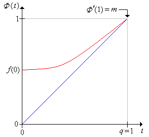
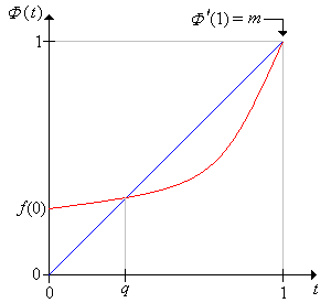
\( q \) is the smallest solution in \( (0, 1] \) of the equation \( \Phi(t) = t \). Moreover
This follows from our analysis of branching chains. The graphs above show the two cases. Note that the condition in (a) means that on average, one or fewer new customers arrive for each customer served. The condition in (b) means that on average, more than one new customer arrives for each customer served.
Our next goal is to find conditions for the queuing chain to be positive recurrent. Recall that \( m \) is the mean of the probability density function \( f \); that is, the expected number of new customers who arrive during a time period. As before, let \( \tau_0 \) denote the first positive time that the chain is in state 0. We assume that the chain is recurrent, so \( m \le 1 \) and \( \P(\tau_0 \lt \infty) = 1 \).
Let \( \Psi \) denote the probability generating function of \( \tau_0 \), starting in state 1. Then
\( \Psi(t) = t \Phi[\Psi(t)] \) for \( t \in [-1, 1] \).
Once again, the trick is to condition on the first state: \[ \Psi(t) = \E\left(t^{\tau_0} \bigm| X_0 = 1\right) = \sum_{x = 0}^\infty \E\left(t^{\tau_0} \bigm| X_0 = 1, X_1 = x\right) \P(X_1 = x \mid X_0 = 1) \] First note that \( \E\left(t^{\tau_0} \bigm| X_0 = 1, X_1 = 0\right) = t^1 = t \Psi^0(t) \). On the other hand, by the Markov property and , \[ \E\left(t^{\tau_0} \bigm| X_0 = 1, X_1 = x\right) = \E\left(t^{1 + \tau_0} \bigm| X_0 = x\right) = t \E\left(t^{\tau_0} \bigm| X_0 = x\right) = t \Psi^x(t), \quad x \in \N_+ \] Of course \( \P(X_1 = x \mid X_0 = 1) = P(1, x) = f(x) \). Hence we have \[ \Psi(t) = \sum_{x=0}^\infty t \Psi^x(t) f(x) = t \Phi[\Psi(t)] \] The PGF of any variable that takes positive integer values is defined on \( [-1, 1] \), and maps this interval back into itself. Hence the representation is valid at least for \( t \in [-1, 1] \).
The deriviative of \( \Psi \) is \[ \Psi^\prime(t) = \frac{\Phi[\Psi(t)]}{1 - t \Phi^\prime[\Psi(t)]}, \quad t \in (-1, 1) \]
As usual, let \( \mu_0 = \E(\tau_0 \mid X_0 = 0) \), the mean return time to state 0 starting in state 0. Then
Recall that \( \Psi \) is the probability generating function of \( \tau_0 \), starting at 0. From basic properties of PGFs we know that \( \Phi(t) \uparrow 1 \), \( \Psi(t) \uparrow 1 \), \( \Phi^\prime(t) \uparrow m \), and \( \Psi^\prime(t) \uparrow \mu_0 \) as \( t \uparrow 1 \). So letting \( t \uparrow 1 \) in the result of the previous theorem, we have \( \mu_0 = 1 \big/ (1 - m) \) if \( m \lt 1 \) and \( \mu_0 = \infty \) if \( m = 1 \).
So to summarize, the queuing chain is positive recurrent if \( m \lt 1 \), null recurrent if \( m = 1 \), and transient if \( m > 1 \). Since \( m \) is the expected number of new customers who arrive during a service period, the results are certainly reasonable.
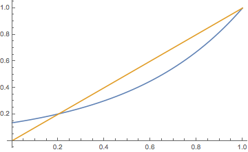
Consider the queuing chain with arrival probability density function \( f \) given by \( f(0) = 1 - p \), \( f(2) = p \), where \( p \in (0, 1) \) is a parameter. Thus, at each time period, either no new customers arrive or two arrive.
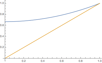
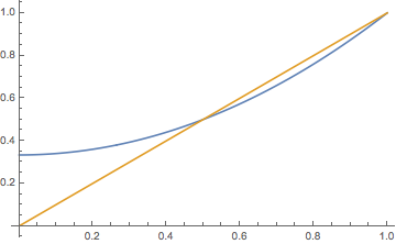
Consider the queuing chain whose arrival distribution is the geometric distribution on \( \N \) with parameter \( 1 - p \), where \( p \in (0, 1) \). Thus \( f(n) = (1 - p) p^n \) for \( n \in \N \).
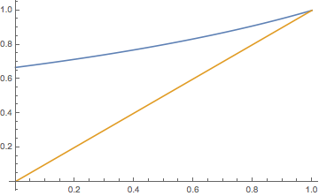
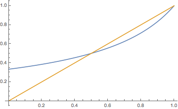
Curiously, the parameter \( q \) and the classification of the chain are the same as in .
Consider the queuing chain whose arrival distribution is the Poisson distribution with parameter \( m \in (0, \infty) \). Thus \( f(n) = e^{-m} m^n / n! \) for \( n \in \N \). Find each of the following:

