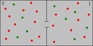
The Bernoulli-Laplace chain, named for Jacob Bernoulli and Pierre Simon Laplace, is a simple discrete model for the diffusion of two incompressible gases between two containers. Like the Ehrenfest chain, it can also be formulated as a simple ball and urn model. Thus, suppose that we have two urns, labeled 0 and 1. Urn 0 contains \( j \) balls and urn 1 contains \( k \) balls, where \( j, \, k \in \N_+ \). Of the \( j + k \) balls, \( r \) are red and the remaining \( j + k - r \) are green. Thus \( r \in \N_+ \) and \( 0 \lt r \lt j + k \). At each discrete time, independently of the past, a ball is selected at random from each urn and then the two balls are switched. The balls of different colors correspond to molecules of different types, and the urns are the containers. The incompressible property is reflected in the fact that the number of balls in each urn remains constant over time.

Let \( X_n \) denote the number of red balls in urn 1 at time \( n \in \N \). Then
\( \bs{X} = (X_0, X_1, X_2, \ldots) \) is a discrete-time Markov chain with state space \( S = \{\max\{0, r - j\}, \ldots, \min\{k,r\}\} \) and with transition matrix \( P \) given by \[ P(x, x - 1) = \frac{(j - r + x) x}{j k}, \; P(x, x) = \frac{(r - x) x + (j - r + x)(k - x)}{j k}, \; P(x, x + 1) = \frac{(r - x)(k - x)}{j k}; \quad x \in S \]
For the state space, note from that the number of red balls \( x \) in urn 1 must satisfy the inequalities \( x \ge 0 \), \( x \le k \), \( x \le r \), and \( x \ge r - j \). The Markov property is clear from the model. For the transition probabilities, note that to go from state \( x \) to state \(x - 1 \) we must select a green ball from urn 0 and a red ball from urn 1. The probabilities of these events are \( (j - r + x) / j \) and \( x / k \) for \( x \) and \( x - 1 \) in \( S \), and the events are independent. Similarly, to go from state \( x \) to state \( x + 1 \) we must select a red ball from urn 0 and a green ball from urn 1. The probabilities of these events are \( (r - x) / j \) and \( (k - x) / k \) for \( x \) and \( x + 1 \) in \( S \), and the events are independent. Finally, to go from state \( x \) back to state \( x \), we must select a red ball from both urns or a green ball from both urns. Of course also, \( P(x, x) = 1 - P(x, x - 1) - P(x, x + 1) \).
This is a fairly complicated model, simply because of the number of parameters. Interesting special cases occur when some of the parameters are the same.
Consider the special case \( j = k \), so that each urn has the same number of balls. The state space is \( S = \{\max\{0, r - k\}, \ldots, \min\{k,r\}\} \) and the transition probability matrix is \[ P(x, x - 1) = \frac{(k - r + x) x}{k^2}, \; P(x, x) = \frac{(r - x) x + (k - r + x)(k - x)}{k^2}, \; P(x, x + 1) = \frac{(r - x)(k - x)}{k^2}; \quad x \in S \]
Consider the special case \( r = j \), so that the number of red balls is the same as the number of balls in urn 0. The state space is \( S = \{0, \ldots, \min\{j, k\}\} \) and the transition probability matrix is \[ P(x, x - 1) = \frac{x^2}{j k}, \; P(x, x) = \frac{x (j + k - 2 x)}{j k}, \; P(x, x + 1) = \frac{(j - x)(k - x)}{j k}; \quad x \in S \]
Consider the special case \( r = k \), so that the number of red balls is the same as the number of balls in urn 1. The state space is \( S = \{\max\{0, k - j\}, \ldots, k\} \) and the transition probability matrix is \[ P(x, x - 1) = \frac{(j - k + x) x}{j k}, \; P(x, x) = \frac{(k - x)(j - k + 2 x)}{j k}, \; P(x, x + 1) = \frac{(k - x)^2}{j k}; \quad x \in S \]
Consider the special case \( j = k = r \), so that each urn has the same number of balls, and this is also the number of red balls. The state space is \( S = \{0, 1, \ldots, k\} \) and the transition probability matrix is \[ P(x, x - 1) = \frac{x^2}{k^2}, \; P(x, x) = \frac{2 x (k - x)}{k^2}, \; P(x, x + 1) = \frac{(k - x)^2}{k^2}; \quad x \in S \]
Run the simulation of the Bernoulli-Laplace experiment for 10000 steps and for various values of the parameters. Note the limiting behavior of the proportion of time spent in each state.
The Bernoulli-Laplace chain is irreducible.
Note that \( P(x, x - 1) \gt 0 \) whenever \( x, \, x - 1 \in S \), and \( P(x, x + 1) \gt 0 \) whenever \( x, \, x + 1 \in S \). Hence every state leads to every other state so the chain is irreducible.
Except in the trivial case \( j = k = r = 1 \), the Bernoulli-Laplace chain aperiodic.
Consideration of the state probabilities shows that except when \( j = k = r = 1 \), the chain has a state \( x \) with \( P(x, x) \gt 0 \), so state \( x \) is aperiodic. Since the chain is irreducible by the previous result, all states are aperiodic.
The invariant distribution is the hypergeometric distribution with population parameter \( j + k \), sample parameter \( k \), and type parameter \( r \). The probability density function is \[ f(x) = \frac{\binom{r}{x} \binom{j + k - r}{k - x}}{\binom{j + k}{k}}, \quad x \in S \]
Thus, the invariant distribution corresponds to selecting a sample of \( k \) balls at random and without replacement from the \( j + k \) balls and placing them in urn 1. The mean and variance of the invariant distribution are \[ \mu = k \frac{r}{j + k}, \; \sigma^2 = k \frac{r}{j + k} \frac{j + k - r}{j + k} \frac{j}{j + k -1} \]
The mean return time to each state \( x \in S \) is \[ \mu(x) = \frac{\binom{j + k}{k}}{\binom{r}{x} \binom{j + k - r}{k - x}} \]
\( P^n(x, y) \to f(y) = \binom{r}{y} \binom{r + k - r}{k - y} \big/ \binom{j + k}{k} \) as \( n \to \infty \) for \( (x, y) \in S^2 \).
In the simulation of the Bernoulli-Laplace experiment, vary the parameters and note the shape and location of the limiting hypergeometric distribution. For selected values of the parameters, run the simulation for 10000 steps and and note the limiting behavior of the proportion of time spent in each state.
The Bernoulli-Laplace chain is reversible.
Let \[ g(x) = \binom{r}{x} \binom{j + k - r}{k - x}, \quad x \in S \] It suffices to show the reversibility condition \( g(x) P(x, y) = g(y) P(y, x) \) for all \( x, \, y \in S \). It then follows that \( \bs{X} \) is reversible and that \( g \) is invariant for \( \bs{X} \). For \( x \in S \) and \( y = x - 1 \in S \), the left and right sides of the reversibility condition reduce to \[ \frac{1}{j k}\frac{r!}{(x - 1)! (r - x)!} \frac{(j + k - r)!}{(k - x)! (j - r + x - 1)!} \] For \( x \in S \) and \( y = x + 1 \in S \), the left and right sides of the reversibility condition reduce to \[ \frac{1}{j k} \frac{r!}{x! (r - x - 1)!} \frac{(j + k - r)!}{(k - x - 1)! (j - r + x)!} \] For all other values of \( x, \, y \in S \), the reversibility condition is trivially satisfied. The hypergeometric PDF \( f \) in is simply \( g \) normalized, so this proves that \( f \) is also invariant.
Run the simulation of the Bernoulli-Laplace experiment 10,000 time steps for selected values of the parameters, and with initial state 0. Note that at first, you can see the arrow of time
. After a long period, however, the direction of time is no longer evident.
Consider the Bernoulli-Laplace chain with \( j = 10 \), \( k = 5 \), and \( r = 4 \). Suppose that \( X_0 \) has the uniform distribution on \( S \). Explicitly give each of the following:
Consider the Bernoulli-Laplace chain with \( j = k = 10 \) and \( r = 6 \). Give each of the following explicitly: