The Markov property, stated in the form that the past and future are independent given the present, essentially treats the past and future symmetrically. However, there is a lack of symmetry in the fact that in the usual formulation, we have an initial time 0, but not a terminal time. If we introduce a terminal time, then we can run the process backwards in time. In this section, we are interested in the following questions:
Consideration of these questions leads to reversed chains, an important and interesting part of the theory of Markov chains.
Our starting point is a (homogeneous) discrete-time Markov chain \( \bs{X} = (X_0, X_1, X_2, \ldots) \) with (countable) state space \( S \) and transition probability matrix \( P \). Let \( m \) be a positive integer, which we will think of as the terminal time or finite time horizon. We won't bother to indicate the dependence on \( m \) notationally, since ultimately the terminal time will not matter. Define \( \hat X_n = X_{m-n} \) for \( n \in \{0, 1, \ldots, m\} \). Thus, the process forward in time is \( \bs{X} = (X_0, X_1, \ldots, X_m) \) while the process backwards in time is \[ \hat{\bs X} = (\hat X_0, \hat X_1, \ldots, \hat X_m) = (X_m, X_{m-1}, \ldots, X_0) \]
For \( n \in \{0, 1, \ldots, m\} \), let \[ \hat{\mathscr F}_n = \sigma\{\hat X_0, \hat X_1, \ldots, \hat X_n\} = \sigma\{X_{m-n}, X_{m - n + 1}, \ldots, X_m\} \] denote the \( \sigma \) algebra of the events of the process \( \hat{\bs X} \) up to time \( n \). So of course, an event for \( \hat{\bs X} \) up to time \( n \) is an event for \( \bs X \) from time \( m - n \) forward. Our first result is that the reversed process is still a Markov chain, but not time homogeneous in general.The process \( \hat{\bs X} = (\hat X_0, \hat X_1, \ldots, \hat X_m) \) is a Markov chain, but is not time homogenous in general. The one-step transition matrix at time \( n \in \{0, 1, \ldots, m - 1\} \) is given by \[ \P(\hat X_{n+1} = y \mid \hat X_n = x) = \frac{\P(X_{m - n - 1} = y)}{\P(X_{m - n} = x)} P(y, x), \quad (x, y) \in S^2\]
Let \( A \in \hat{\mathscr F}_n \) and \( x, \, y \in S \). Then \begin{align*} \P(\hat X_{n+1} = y \mid \hat X_n = x, A) & = \frac{\P(\hat X_{n+1} = y, \hat X_n = x, A)}{\P(\hat X_n = x, A)} = \frac{\P(X_{m - n - 1} = y, X_{m - n} = x, A)}{\P(X_{m - n} = x, A)} \\ & = \frac{\P(A \mid X_{m - n - 1} = y, X_{m - n} = x) \P(X_{m - n} = x \mid X_{m - n - 1} = y) \P(X_{m - n - 1} = y)}{\P(A \mid X_{m - n} = x) \P(X_{m - n} = x)} \end{align*} But \( A \in \sigma\{X_{m - n}, \ldots, X_m\} \) and so by the Markov property for \( \bs X \), \[ \P(A \mid X_{m - n - 1} = y, X_{m - n} = x) = \P(A \mid X_{m - n} = x) \] By the time homogeneity of \( \bs X \), \(\P(X_{m - n} = x \mid X_{m - n - 1} = y) = P(y, x)\). Substituting and simplifying gives \[ \P(\hat X_{n+1} = y \mid \hat X_n = x, A) = \frac{\P(X_{m - n - 1} = y)}{\P(X_{m - n} = x)} P(y, x) \]
However, the backwards chain will be time homogeneous if \( X_0 \) has an invariant distribution.
Suppose that \( \bs X \) is irreducible and positive recurrent, with (unique) invariant probability density function \( f \). If \( X_0 \) has the invariant probability distribution, then \( \hat{\bs X} \) is a time-homogeneous Markov chain with transition matrix \( \hat P \) given by \[ \hat P(x, y) = \frac{f(y)}{f(x)} P(y, x), \quad (x, y) \in S^2 \]
Recall that a discrete-time Markov chain is ergodic if it is irreducible, positive recurrent, and aperiodic. For an ergodic chain, holds in the limit of the terminal time.
Suppose that \( \bs X \) is ergodic, with (unique) invariant probability density function \( f \). Regardless of the distribution of \( X_0 \), \[\P(\hat X_{n+1} = y \mid \hat X_n = x) \to \frac{f(y)}{f(x)} P(y, x) \text{ as } m \to \infty\]
This follows from the conditional probability in and our study of the limiting behavior of Markov chains. Since \( \bs X \) is ergodic, \( \P(X_k = x) \to f(x) \) as \( k \to \infty \) for every \( x \in S \).
These three results are motivation for the definition that follows. We can generalize by defining the reversal of an irreducible Markov chain, as long as there is a positive, invariant function. Recall that a positive invariant function defines a positive measure on \( S \), but of course not in general a probability distribution.
Suppose that \( \bs X \) is an irreducible Markov chain with transition matrix \( P \), and that \( g: S \to (0, \infty) \) is invariant for \( \bs X \). The reversal of \( \bs X \) with respect to \( g \) is the Markov chain \( \hat{\bs X} = (\hat X_0, \hat X_1, \ldots) \) with transition probability matrix \( \hat P \) defined by \[\hat P(x, y) = \frac{g(y)}{g(x)} P(y, x), \quad (x, y) \in S^2\]
We need to show that \( \hat P \) is a valid transition probability matrix, so that the definition makes sense. Since \( g \) is invariant for \( \bs X \), \[\sum_{y \in S} \hat P(x, y) = \frac{1}{g(x)} \sum_{y \in S} g(y) P(y, x) = \frac{g(x)}{g(x)} = 1, \quad x \in S\]
Recall that if \( g \) is a positive invariant function for \( \bs X \) then so is \( c g \) for every positive constant \( c \). Note that \( g \) and \( c g \) generate the same reversed chain. So let's consider the cases:
Suppose that \( \bs X \) is an irreducible Markov chain on \( S \).
Nonetheless, definition is natural, because most of the important properties of the reversed chain follow from the balance equation between the transition matrices \( P \) and \( \hat P \), and the invariant function \( g \): \[ g(x) \hat P(x, y) = g(y) P(y, x), \quad (x, y) \in S^2 \] We will see this balance equation repeated with other objects related to the Markov chains.
Suppose that \( \bs X \) is an irreducible Markov chain with invariant function \( g: S \to (0, \infty) \), and that \( \hat{\bs X} \) is the reversal of \( \bs X \) with respect to \( g \). For \( x, \, y \in S \),
These results follow immediately from the balance equation \( g(x) \hat P(x, y) = g(y) P(y, x) \) for \( (x, y) \in S^2 \).
From part (b) of it follows that the state graphs of \( \bs X \) and \( \hat{\bs X} \) are reverses of each other. That is, to go from the state graph of one chain to the state graph of the other, simply reverse the direction of each edge. Here is a more complicated (but equivalent) version of the balance equation for chains of states:
Suppose again that \( \bs X \) is an irreducible Markov chain with invariant function \( g: S \to (0, \infty) \), and that \( \hat{\bs X} \) is the reversal of \( \bs X \) with respect to \( g \). For every \( n \in \N_+ \) and every sequence of states \( (x_1, x_2, \ldots, x_n, x_{n+1}) \in S^{n+1} \), \[ g(x_1) \hat P(x_1, x_2) \hat P(x_2, x_3) \cdots \hat P(x_n, x_{n+1}) = g(x_{n+1}) P(x_{n+1}, x_n) \cdots P(x_3, x_2) P(x_2, x_1) \]
This follows from repeated applications of the basic equation. When \( n = 1 \), we have the balance equation itself: \[g(x_1) \hat P(x_1, x_2) = g(x_2) P(x_2, x_1)\] For \( n = 2 \), \[g(x_1) \hat P(x_1, x_2) \hat P(x_2, x_3) = g(x_2)P(x_2, x_1)\hat P(x_2, x_3) = g(x_3)P(x_3, x_2)P(x_2, x_1)\] Continuing in this manner (or using induction) gives the general result.
The balance equation holds for the powers of the transition matrix:
Suppose again that \( \bs X \) is an irreducible Markov chain with invariant function \( g: S \to (0, \infty) \), and that \( \hat{\bs X} \) is the reversal of \( \bs X \) with respect to \( g \). For every \( (x, y) \in S^2 \) and \( n \in \N \), \[ g(x) \hat P^n(x, y) = g(y) P^n (y, x) \]
When \( n = 0 \), the left and right sides are \( g(x) \) if \( x = y \) and are 0 otherwise. When \( n = 1 \), we have the basic balance equation: \( g(x) \hat P(x, y) = g(y) P(y, x) \). In general, for \( n \in \N_+ \), by we have \begin{align*} g(x) \hat P^n(x, y) &= \sum_{(x_1, \ldots, x_{n-1}) \in S^{n-1}} g(x) \hat P(x, x_1) \hat P(x_1, x_2) \cdots \hat P(x_{n-1}, y) \\ &= \sum_{(x_1, \ldots, x_{n-1}) \in S^{n-1}} g(y) P(y, x_{n-1}) P(x_{n-1}, x_{n-2}) \cdots P(x_1, x) = g(y) P^n(y, x) \end{align*}
Suppose again that \( \bs X \) is an irreducible Markov chain with invariant function \( g: S \to (0, \infty) \), and that \( \hat{\bs X} \) is the reversal of \( \bs X \) with respect to \( g \). For \( n \in \N \) and \( (x, y) \in S^2 \),
In terms of the state graphs, part (b) of has an obvious meaning: If there exists a path of length \( n \) from \( y \) to \( x \) in the original state graph, then there exists a path of length \( n \) from \( x \) to \( y \) in the reversed state graph. The time reversal definition is symmetric with respect to the two Markov chains.
Suppose again that \( \bs X \) is an irreducible Markov chain with invariant function \( g: S \to (0, \infty) \), and that \( \hat{\bs X} \) is the reversal of \( \bs X \) with respect to \( g \). Then
The balance equation also holds for the potential matrices.
Suppose that \( \bs X \) and \( \hat{\bs X} \) are time reversals with respect to the invariant function \( g: S \to (0, \infty) \). For \( \alpha \in (0, 1] \), the \( \alpha \) potential matrices are related by \[ g(x) \hat R_\alpha(x, y) = g(y) R_\alpha(y, x), \quad (x, y) \in S^2 \]
This follows easily from and the definition of the potential matrices: \begin{align*} g(x) \hat R_\alpha(x, y) & = g(x) \sum_{n=0}^\infty \alpha^n \hat P^n(x, y) = \sum_{n=0}^\infty \alpha^n g(x) \hat P^n(x, y) \\ & = \sum_{n=0}^\infty \alpha^n g(y) P^n(y, x) = g(y) \sum_{n=0}^\infty \alpha^n P^n(y, x) = g(y) R_\alpha(y, x) \end{align*}
Markov chains that are time reversals share many important properties:
Suppose that \( \bs X \) and \( \hat{\bs X} \) are time reversals. Then
Suppose that \( \bs X \) and \( \hat{\bs X} \) are time reversals with respect to the invariant function \( g: S \to (0, \infty) \).
The main point of the next result is that we don't need to know a-priori that \( g \) is invariant for \( \bs X \), if we can guess \( g \) and \( \hat P \).
Suppose again that \( \bs X \) is irreducible with transition probability matrix \( P \). If there exists a a function \( g: S \to (0, \infty) \) and a transition probability matrix \( \hat P \) such that \( g(x) \hat P(x, y) = g(y) P(y, x) \) for all \( (x, y) \in S^2 \), then
As a corollary, if there exists a probability density function \( f \) on \( S \) and a transition probability matrix \( \hat P \) such that \( f(x) \hat P(x, y) = f(y) P(y, x) \) for all \( (x, y) \in S^2 \) then in addition to the conclusions above, we know that the chains \( \bs X \) and \( \hat{\bs X} \) are positive recurrent.
Clearly, an interesting special case occurs when the transition matrix of the reversed chain turns out to be the same as the original transition matrix. A chain of this type could be used to model a physical process that is stochastically the same, forward or backward in time.
Suppose again that \( \bs X = (X_0, X_1, X_2, \ldots) \) is an irreducible Markov chain with transition matrix \( P \) and invariant function \( g: S \to (0, \infty) \). If the reversal of \( \bs X \) with respect to \( g \) also has transition matrix \( P \), then \( \bs X \) is said to be reversible with respect to \( g \). That is, \( \bs X \) is reversible with respect to \( g \) if and only if \[ g(x) P(x, y) = g(y) P(y, x), \quad (x, y) \in S^2 \]
Clearly if \( \bs X \) is reversible with respect to the invariant function \( g: S \to (0, \infty) \) then \( \bs X \) is reversible with respect to the invariant function \( c g \) for every \( c \in (0, \infty) \). So again, let's review the cases.
Suppose that \( \bs X \) is an irreducible Markov chain on \( S \).
The non-symmetric simple random walk on \( \Z \) falls into the last case. Using , we can tell whether \( \bs X \) is reversible with respect to \( g \) without knowing a-priori that \( g \) is invariant.
Suppose again that \( \bs X \) is irreducible with transition matrix \( P \). If there exists a function \( g: S \to (0, \infty) \) such that \( g(x) P(x, y) = g(y) P(y, x) \) for all \( (x, y) \in S^2 \), then
If we have reason to believe that a Markov chain is reversible (based on modeling considerations, for example), then the condition in can be used to find the invariant functions. This procedure is often easier than using the definition of invariance directly. The next two results are minor generalizations:
Suppose again that \( \bs X \) is irreducible and that \( g: S \to (0, \infty) \). Then \( g \) is invariant and \( \bs X \) is reversible with respect to \( g \) if and only if for every \( n \in \N_+ \) and every sequence of states \( (x_1, x_2, \ldots x_n, x_{n+1}) \in S^{n+1} \), \[ g(x_1) P(x_1, x_2) P(x_2, x_3) \cdots P(x_n, x_{n+1}) = g(x_{n+1}) P(x_{n+1}, x_n), \cdots P(x_3, x_2) P(x_2, x_1) \]
Suppose again that \( \bs X \) is irreducible and that \( g: S \to (0, \infty) \). Then \( g \) is invariant and \( \bs X \) is reversible with respect to \( g \) if and only if for every \( (x, y) \in S^2 \) and \( n \in \N_+ \), \[ g(x) P^n(x, y) = g(y) P^n(y, x) \]
Here is the condition for reversibility in terms of the potential matrices.
Suppose again that \( \bs X \) is irreducible and that \( g: S \to (0, \infty) \). Then \( g \) is invariant and \( \bs X \) is reversible with respect to \( g \) if and only if \[ g(x) R_\alpha(x, y) = g(y) R_\alpha(y, x), \quad \alpha \in (0, 1], \, (x, y) \in S^2 \]
In the positive recurrent case (the most important case), the following theorem gives a condition for reversibility that does not directly reference the invariant distribution. The condition is known as the Kolmogorov cycle condition, and is named for Andrei Kolmogorov
Suppose that \( \bs X \) is irreducible and positive recurrent. Then \( \bs X \) is reversible if and only if for every sequence of states \( (x_1, x_2, \ldots, x_n) \), \[ P(x_1, x_2) P(x_2, x_3) \cdots P(x_{n-1}, x_n) P(x_n, x_1) = P(x_1, x_n) P(x_n, x_{n-1}) \cdots P(x_3, x_2) P(x_2, x_1) \]
Suppose that \( \bs X \) is reversible. Applying to the sequence \( (x_1, x_2, \ldots, x_n, x_1) \) gives the Kolmogorov cycle condition. Conversely, suppose that the Kolmogorov cycle condition holds, and let \( f \) denote the invariant probability density function of \( \bs X \). From the cycle condition we have \( P(x, y) P^k(y, x) = P(y, x)P^k(x, y) \) for every \( (x, y) \in S \) and \( k \in \N_+ \). Averaging over \( k \) from 1 to \( n \) gives \[ P(x, y) \frac{1}{n} \sum_{k=1}^n P^k(y, x) = P(y, x) \frac{1}{n} \sum_{k = 1}^n P^k(x, y), \quad (x, y) \in S^2, \; n \in \N_+ \]Letting \( n \to \infty \) gives \(f(x) P(x, y) = f(y) P(y, x) \) for \( (x, y) \in S^2 \), so \( \bs X \) is reversible.
Note that the Kolmogorov cycle condition states that the probability of visiting states \( (x_2, x_3, \ldots, x_n, x_1) \) in sequence, starting in state \( x_1 \) is the same as the probability of visiting states \( (x_n, x_{n-1}, \ldots, x_2, x_1) \) in sequence, starting in state \( x_1 \). The cycle condition is also known as the balance equation for cycles.

Recall the general two-state chain \( \bs X \) on \( S = \{0, 1\} \) with the transition probability matrix \[ P = \left[ \begin{matrix} 1 - p & p \\ q & 1 - q \end{matrix} \right] \] where \( p, \, q \in (0, 1) \) are parameters. The chain \( \bs X \) is reversible and the invariant probability density function is \( f = \left( \frac{q}{p + q}, \frac{p}{p + q} \right) \).
All we have to do is note that \[\left[\begin{matrix} q & p \end{matrix}\right] \left[ \begin{matrix} 1 - p & p \\ q & 1 - q \end{matrix} \right] = \left[\begin{matrix} q & p \end{matrix}\right]\]
Open the simulation of the two-state chain. Run the simulation 100 times for various values of \(p\) and \(q\), and different initial states. Note how quickly the arrow of time
is no longer discernable.
Suppose that \( \bs X \) is a Markov chain on a finite state space \( S \) with symmetric transition probability matrix \( P \). Thus \( P(x, y) = P(y, x) \) for all \( (x, y) \in S^2 \). The chain \( \bs X \) is reversible and that the uniform distribution on \( S \) is invariant.
All we have to do is note that \( \bs{1}(x) P(x, y) = \bs{1}(y) P(y, x) \) where \( \bs{1} \) is the constant function 1 on \( S \).
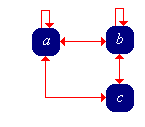
Consider the Markov chain \( \bs X \) on \( S = \{a, b, c\} \) with transition probability matrix \( P \) given below:
\[ P = \left[ \begin{matrix} \frac{1}{4} & \frac{1}{4} & \frac{1}{2} \\ \frac{1}{3} & \frac{1}{3} & \frac{1}{3} \\ \frac{1}{2} & \frac{1}{2} & 0 \end{matrix} \right] \]

Reversibility is discussed in separate sections for each of the following special models: