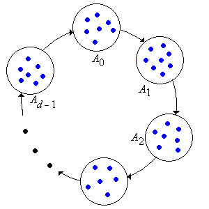
In this section, we study some of the deepest and most interesting parts of the theory of discrete-time Markov chains, involving two different but complementary ideas: stationary distributions and limiting distributions. The theory of renewal processes plays a critical role.
As usual, our starting point is a (time homogeneous) discrete-time Markov chain \( \bs{X} = (X_0, X_1, X_2, \ldots) \) with (countable) state space \( S \) and transition probability matrix \( P \). In the background, of course, is a probability space \( (\Omega, \mathscr{F}, \P) \) so that \( \Omega \) is the sample space, \( \mathscr{F} \) the \( \sigma \)-algebra of events, and \( \P \) the probability measure on \( (\Omega, \mathscr{F}) \). For \( n \in \N \), let \( \mathscr{F}_n = \sigma\{X_0, X_1, \ldots, X_n\} \), the \( \sigma \)-algebra of events determined by the chain up to time \( n \), so that \( \mathfrak{F} = \{\mathscr{F}_0, \mathscr{F}_1, \ldots\}\) is the natural filtration associated with \( \bs{X} \).
Let \( y \in S \) and \( n \in \N_+ \). We will denote the number of visits to \( y \) during the first \( n \) positive time units by \[ N_{y,n} = \sum_{i=1}^n \bs{1}(X_i = y) \] Note that \( N_{y,n} \to N_y \) as \( n \to \infty \), where \[ N_y = \sum_{i=1}^\infty \bs{1}(X_i = y) \] is the total number of visits to \( y \) at positive times, one of the important random variables that we studied in the section on transience and recurrence. For \( n \in \N_+ \), we denote the time of the \( n \)th visit to \( y \) by \[ \tau_{y,n} = \min\{k \in \N_+: N_{y,k} = n\} \] where as usual, we define \( \min(\emptyset) = \infty \). Note that \( \tau_{y,1} \) is the time of the first visit to \( y \), which we denoted simply by \(\tau_y \) in the section on transience and recurrence. The times of the visits to \( y \) are stopping times for \( \bs{X} \). That is, \( \{\tau_{y,n} = k\} \in \mathscr{F}_k \) for \( n \in \N_+ \) and \( k \in \N \). Recall also the definition of the hitting probability to state \( y \) starting in state \( x \): \[ H(x, y) = \P\left(\tau_y \lt \infty \mid X_0 = x\right), \quad (x, y) \in S^2 \]
Suppose that \( x, \, y \in S \), and that \( y \) is recurrent and \( X_0 = x \).
Let \( \tau_{y,0} = 0 \) for convenience.
As noted in the proof, \( \left(\tau_{y,1}, \tau_{y,2}, \ldots\right) \) is the sequence of arrival times and \( \left(N_{y,1}, N_{y,2}, \ldots\right) \) is the associated sequence of counting variables for the embedded renewal process associated with the recurrent state \( y \). The corresponding renewal function, given \( X_0 = x \), is the function \( n \mapsto G_n(x, y) \) where \[ G_n(x, y) = \E\left(N_{y,n} \mid X_0 = x\right) = \sum_{k=1}^n P^k(x, y), \quad n \in \N \] Thus \( G_n(x, y) \) is the expected number of visits to \( y \) in the first \( n \) positive time units, starting in state \( x \). Note that \( G_n(x, y) \to G(x, y) \) as \( n \to \infty \) where \( G \) is the potential matrix that we studied previously. This matrix gives the expected total number visits to state \( y \in S \), at positive times, starting in state \( x \in S \): \[ G(x, y) = \E\left(N_y \mid X_0 = x\right) = \sum_{k=1}^\infty P^k(x, y) \]
The limit theorems of renewal theory can now be used to explore the limiting behavior of the Markov chain. Let \( \mu(y) = \E(\tau_y \mid X_0 = y) \) denote the mean return time to state \( y \), starting in \( y \). In the following results, it may be the case that \( \mu(y) = \infty \), in which case we interpret \( 1 / \mu(y) \) as 0.
If \( x, \, y \in S \) and \( y \) is recurrent then \[ \P\left( \frac{1}{n} N_{n,y} \to \frac{1}{\mu(y)} \text{ as } n \to \infty \biggm| X_0 = x \right) = H(x, y) \]
This result follows from the strong law of large numbers for renewal processes.
Note that \( \frac{1}{n} N_{y,n} = \frac{1}{n} \sum_{k=1}^n \bs{1}(X_k = y) \) is the average number of visits to \( y \) in the first \( n \) positive time units.
If \( x, \, y \in S \) and \( y \) is recurrent then \[ \frac{1}{n} G_n(x, y) = \frac{1}{n} \sum_{k=1}^n P^k(x, y) \to \frac{H(x, y)}{\mu(y)} \text{ as } n \to \infty \]
This result follows from the elementary renewal theorem for renewal processes.
Note that \( \frac{1}{n} G_n(x, y) = \frac{1}{n} \sum_{k=1}^n P^k(x, y) \) is the expected average number of visits to \( y \) during the first \( n \) positive time units, starting at \( x \).
If \( x, \, y \in S \) and \( y \) is recurrent and aperiodic then \[ P^n(x, y) \to \frac{H(x, y)}{\mu(y)} \text{ as } n \to \infty \]
This result follows from the renewal theorem for renewal processes.
Note that \( H(y, y) = 1 \) by the very definition of a recurrent state. Thus, when \( x = y \), gives convergence with probability 1, and the limits in and are simply \( 1 / \mu(y) \). By contrast, we already know the corresponding limiting behavior when \( y \) is transient.
If \(x, \, y \in S \) and \( y \) is transient then
On the other hand, if \( y \) is transient then \( \P(\tau_y = \infty \mid X_0 = y) \gt 0 \) by the very definition of a transience. Thus \( \mu(y) = \infty \), and so the results in parts (b) and (c) agree with the corresponding results above for a recurrent state. Here is a summary.
For \( x, \, y \in S \), \[ \frac{1}{n} G_n(x, y) = \frac{1}{n} \sum_{k=1}^n P^k(x, y) \to \frac{H(x, y)}{\mu(y)} \text{ as } n \to \infty \] If \( y \) is transient or if \( y \) is recurrent and aperiodic, \[ P^n(x, y) \to \frac{H(x, y)} {\mu(y)} \text{ as } n \to \infty \]
Clearly there is a fundamental dichotomy in terms of the limiting behavior of the chain, depending on whether the mean return time to a given state is finite or infinite. Thus the following definition is natural.
Let \( x \in S \).
Implicit in the definition is the following simple result:
If \( x \in S \) is positive recurrent, then \( x \) is recurrent.
Recall that if \( \E(\tau_x \mid X_0 = x) \lt \infty \) then \( \P(\tau_x \lt \infty \mid X_0 = x) = 1 \).
On the other hand, it is possible to have \( \P(\tau_x \lt \infty \mid X_0 = x) = 1 \), so that \( x \) is recurrent, and also \( \E(\tau_x \mid X_0 = x) = \infty \), so that \( x \) is null recurrent. Simply put, a random variable can be finite with probability 1, but can have infinite expected value. A classic example is the Pareto distribution with shape parameter \( a \in (0, 1) \).
Like recurrence/transience, and period, the null/positive recurrence property is a class property.
If \( x \) is positive recurrent and \( x \to y \) then \( y \) is positive recurrent.
Suppose that \( x \) is positive recurrent and \( x \to y \). Recall that \( y \) is recurrent and \( y \to x \). Hence there exist \( i, \, j \in \N_+ \) such that \( P^i(x, y) \gt 0 \) and \( P^j(y, x) \gt 0 \). Thus for every \( k \in \N_+ \), \( P^{i+j+k}(y, y) \ge P^j(y, x) P^k(x, x) P^i(x, y) \). Averaging over \( k \) from 1 to \( n \) gives \[ \frac{G_n(y, y)}{n } - \frac{G_{i+j}(y, y)}{n} \ge P^j(y, x) \frac{G_n(x, x)}{n} P^i(x, y)\] Letting \( n \to \infty \) and using gives \[ \frac{1}{\mu(y)} \ge P^j(y, x) \frac{1}{\mu(x)} P^i(x, y) \gt 0 \] Therefore \( \mu(y) \lt \infty \) and so \( y \) is also positive recurrent.
Thus, the terms positive recurrent and null recurrent can be applied to equivalence classes (under the to and from equivalence relation), as well as individual states. When the chain is irreducible, the terms can be applied to the chain as a whole.
Recall that a nonempty set of states \( A \) is closed if \( x \in A \) and \( x \to y \) implies \( y \in A \). Here are some simple results for a finite, closed set of states.
If \( A \subseteq S \) is finite and closed, then \( A \) contains a positive recurrent state.
Fix a state \( x \in A \) and note that \( P^k(x, A) = \sum_{y \in A} P^k(x, y) = 1 \) for every \( k \in \N_+ \) since \( A \) is closed. Averaging over \( k \) from 1 to \( n \) gives \[ \sum_{y \in A} \frac{G_n(x, y)}{n} = 1 \] for every \( n \in \N_+ \). Note that the change in the order of summation is justified since both sums are finite. Assume now that all states in \( A \) are transient or null recurrent. Letting \( n \to \infty \) in the displayed equation gives the contradiction \( 0 = 1 \). Again, the interchange of sum and limit is justified by the fact that \( A \) is finite.
If \( A \subseteq S \) is finite and closed, then \( A \) contains no null recurrent states.
Let \( x \in A \). Note that \( [x] \subseteq A \) since \( A \) is closed. Suppose that \( x \) is recurrent. Note that \( [x] \) is also closed and finite and hence must have a positive recurrent state by . Hence the equivalence class \( [x] \) is positive recurrent and thus so is \( x \).
If \( A \subseteq S \) is finite and irreducible, then \( A \) is a positive recurrent equivalence class.
In particular, a Markov chain with a finite state space cannot have null recurrent states; every state must be transient or positive recurrent.
Returning to the limiting behavior, suppose that the chain \( \bs{X} \) is irreducible, so that either all states are transient, all states are null recurrent, or all states are positive recurrent. From , if the chain is transient or if the chain is recurrent and aperiodic, then \[ P^n(x, y) \to \frac{1}{\mu(y)} \text{ as } n \to \infty \text{ for every } x \in S \] Note in particular that the limit is independent of the initial state \( x \). Of course in the transient case and in the null recurrent and aperiodic case, the limit is 0. Only in the positive recurrent, aperiodic case is the limit positive, which motivates our next definition.
A Markov chain \( \bs{X} \) that is irreducible, positive recurrent, and aperiodic, is said to be ergodic.
The behavior when the chain is periodic with period \( d \in \{2, 3, \ldots\} \) is a bit more complicated, but we can understand this behavior by considering the \( d \)-step chain \( \bs{X}_d = (X_0, X_d, X_{2 d}, \ldots) \) that has transition matrix \( P^d \). Essentially, this allows us to trade periodicity (one form of complexity) for reducibility (another form of complexity). Specifically, recall that the \( d \)-step chain is aperiodic but has \( d \) equivalence classes \( (A_0, A_1, \ldots, A_{d-1}) \); and these are the cyclic classes of original chain \( \bs{X} \).

The mean return time to state \( x \) for the \( d \)-step chain \( \bs{X}_d \) is \( \mu_d(x) = \mu(x) / d \).
Note that every single step for the \( d \)-step chain corresponds to \( d \) steps for the original chain.
Let \( i, \, j, \, k \in \{0, 1, \ldots, d - 1\} \),
If \( y \in S \) is null recurrent or transient then regardless of the period of \( y \), \( P^n(x, y) \to 0 \) as \( n \to \infty \) for every \( x \in S \).
Our next goal is to see how the limiting behavior is related to invariant distributions. Suppose that \( f \) is a probability density function on the state space \( S \). Recall that \( f \) is invariant for \( P \) (and for the chain \( \bs{X} \)) if \( f P = f \). It follows immediately that \( f P^n = f \) for every \( n \in \N \). Thus, if \( X_0 \) has probability density function \( f \) then so does \( X_n \) for each \( n \in \N \), and hence \( \bs{X} \) is a sequence of identically distributed random variables. A bit more generally, suppose that \( g: S \to [0, \infty) \) is invariant for \( P \), and let \( C = \sum_{x \in S} g(x) \). If \( 0 \lt C \lt \infty \) then \( f \) defined by \( f(x) = g(x) / C \) for \( x \in S \) is an invariant probability density function.
Suppose that \( g: S \to [0, \infty) \) is invariant for \( P \) and satisfies \( \sum_{x \in S} g(x) \lt \infty \). Then \[ g(y) = \frac{1}{\mu(y)} \sum_{x \in S} g(x) H(x, y), \quad y \in S \]
Recall again that \( g P^k = g \) for every \( k \in \N \) since \( g \) is invariant for \( P \). Averaging over \( k \) from 1 to \( n \) gives \( g G_ n / n = g \) for each \( n \in \N_+ \). Explicitly, \[ \sum_{x \in S} g(x) \frac{G_n(x, y)}{n} = g(y), \quad y \in S \] Letting \( n \to \infty \) and using gives the result. The dominated convergence theorem justifies interchanging the limit with the sum, since the terms are positive, \( \frac{1}{n}G_n(x, y) \le 1 \), and \( \sum_{x \in S} g(x) \lt \infty \).
Note that if \( y \) is transient or null recurrent, then \( g(y) = 0 \). Thus, a invariant function with finite sum, and in particular an invariant probability density function must be concentrated on the positive recurrent states.
Suppose now that the chain \( \bs{X} \) is irreducible. If \( \bs{X} \) is transient or null recurrent, then from the previous result, the only nonnegative functions that are invariant for \( P \) are functions that satisfy \( \sum_{x \in S} g(x) = \infty \) and the function that is identically 0: \( g = \bs{0} \). In particular, the chain does not have an invariant distribution. On the other hand, if the chain is positive recurrent, then \( H(x, y) = 1 \) for all \( x, \, y \in S \). Thus, from the previous result, the only possible invariant probability density function is the function \( f \) given by \( f(x) = 1 / \mu(x) \) for \( x \in S \). Any other nonnegative function \( g \) that is invariant for \( P \) and has finite sum, is a multiple of \( f \) (and indeed the multiple is sum of the values). Our next goal is to show that \( f \) really is an invariant probability density function.
If \( \bs{X} \) is an irreducible, positive recurrent chain then the function \( f \) given by \( f(x) = 1 / \mu(x) \) for \( x \in S \) is an invariant probability density function for \( \bs{X} \).
Let \( f(x) = 1 / \mu(x) \) for \( x \in S \), and let \( A \) be a finite subset of \( S \). Then \( \sum_{y \in A} \frac{1}{n} G_n(x, y) \le 1 \) for every \( x \in S \). Letting \( n \to \infty \) and using gives \( \sum_{y \in A} f(y) \le 1 \). The interchange of limit and sum is justified since \( A \) is finite. Since this is true for every finite \( A \subseteq S \), it follows that \( C \le 1 \) where \( C = \sum_{y \in S} f(y) \). Note also that \( C \gt 0 \) since the chain is positive recurrent. Next note that \[ \sum_{y \in A} \frac{1}{n} G_n(x, y) P(y, z) \le \frac{1}{n} G_{n+1}(x, z) \] for every \( x, \, z \in S \). Letting \( n \to \infty \) gives \( \sum_{y \in A} f(y) P(y, z) \le f(z) \) for every \( z \in S \). It then follows that \( \sum_{y \in S} f(y) P(y, z) \le f(z) \) for every \( z \in S \). Suppose that strict inequality holds for some for some \( z \in S \). Then \[ \sum_{z \in S} \sum_{y \in S} f(y) P(y, z) \lt \sum_{z \in S} f(z) \] Interchanging the order of summation on the left in the displayed inequality yields the contradiction \( C \lt C \). Thus \( f \) is invariant for \( P \). Hence \( f / C \) is an invariant probability density function. By the uniqueness result noted earlier, it follows that \( f / C = f \) so that in fact \( C = 1 \).
In summary, an irreducible, positive recurrent Markov chain \( \bs{X} \) has a unique invariant probability density function \( f \) given by \( f(x) = 1 / \mu(x) \) for \( x \in S \). We also now have a test for positive recurrence. An irreducible Markov chain \( \bs{X} \) is positive recurrent if and only if there exists a positive function \( g \) on \( S \) that is invariant for \( P \) and satisfies \( \sum_{x \in S} g(x) \lt \infty \) (and then, of course, normalizing \( g \) would give \( f \)).
Consider now a general Markov chain \( \bs{X} \) on \( S \). If \( \bs{X} \) has no positive recurrent states, then as noted earlier, there are no invariant distributions. Thus, suppose that \( \bs{X} \) has a collection of positive recurrent equivalence classes \( (A_i: i \in I) \) where \( I \) is a nonempty, countable index set. The chain restricted to \( A_i \) is irreducible and positive recurrent for each \( i \in I \), and hence has a unique invariant probability density function \( f_i \) on \( A_i \) given by \[ f_i(x) = \frac{1}{\mu(x)}, \quad x \in A_i \] We extend \( f_i \) to \( S \) by defining \( f_i(x) = 0 \) for \( x \notin A_i \), so that \( f_i \) is a probability density function on \( S \). All invariant probability density functions for \( \bs{X} \) are mixtures of these functions:
\( f \) is an invariant probability density function for \( \bs{X} \) if and only if \( f \) has the form \[ f(x) = \sum_{i \in I} p_i f_i(x), \quad x \in S \] where \( (p_i: i \in I) \) is a probability density function on the index set \( I \). That is, \( f(x) = p_i f_i(x) \) for \( i \in I \) and \( x \in A_i \), and \( f(x) = 0 \) otherwise.
Let \( A = \bigcup_{i \in I} A_i \), the set of positive recurrent states. Suppose that \( f \) has the form given in the theorem. Since \( f(x) = 0 \) for \( x \notin A \) we have \[(f P)(y) = \sum_{x \in S} f(x) P(x, y) = \sum_{i \in I} \sum_{x \in A_i} p_i f_i(x) P(x, y)\] Suppose that \( y \in A_j \) for some \( j \in I \). Since \( P(x, y) = 0 \) if \( x \in A_i \) and \( i \ne j \), the last sum becomes \[(f P)(y) = p_j \sum_{x \in A_j} f_j(x) P(x, y) = p_j f_j(y) = f(y)\] because \( f_j \) is invariant for the \( P \) restricted to \( A_j \). If \( y \notin A \) then \( P(x, y) = 0 \) for \( x \in A \) so the sum above becomes \( (f P)(y) = 0 = f(y) \). Hence \( f \) is invariant. Moreover, \[\sum_{x \in S} f(x) = \sum_{i \in I} \sum_{x \in A_i} f(x) = \sum_{i \in I} p_i \sum_{x \in A_i} f_i(x) = \sum_{i \in I} p_i = 1\] so \( f \) is a PDF on \( S \). Conversely, suppose that \( f \) is an invariant PDF for \( \bs{X} \). We know that \( f \) is concentrated on the positive recurrent states, so \( f(x) = 0 \) for \( x \notin A\). For \( i \in I \) and \( y \in A_i \) \[\sum_{x \in A_i} f(x) P(x, y) = \sum_{x \in S} f(x) P(x, y) = f(y)\] since \( f \) is invariant for \( P \) and since, as noted before, \( f(x) P(x, y) = 0 \) if \( x \notin A_i \). It follows that \( f \) restricted to \( A_i \) is invariant for the chain restricted to \( A_i \) for each \( i \in I \). Let \( p_i = \sum_{x \in A_i} f(x) \), the normalizing constant for \( f \) restricted to \( A_i \). By uniqueness, the restriction of \( f / p_i \) to \( A_i \) must be \( f_i \), so \( f \) has the form given in the theorem.
Suppose that \( \bs{X} \) is irreducible. In this section we are interested in general functions \( g: S \to [0, \infty) \) that are invariant for \( \bs{X} \), so that \( g P = g \). A function \( g: S \to [0, \infty) \) defines a positive measure \( \nu \) on \( S \) by the simple rule \[ \nu(A) = \sum_{x \in A} g(x), \quad A \subseteq S \] so in this sense, we are interested in invariant positive measures for \( \bs{X} \) that may not be probability measures. Technically, \( g \) is the density function of \( \nu \) with respect to counting measure \( \# \) on \( S \).
From our work above, We know the situation if \( \bs{X} \) is positive recurrent. In this case, there exists a unique invariant probability density function \( f \) that is positive on \( S \), and every other nonnegative invariant function \( g \) is a nonnegative multiples of \( f \). In particular, either \( g = \bs{0} \), the zero function on \( S \), or \( g \) is positive on \( S \) and satisfies \( \sum_{x \in S} g(x) \lt \infty \).
We can generalize to chains that are simply recurrent, either null or positive. We will show that there exists a positive invariant function that is unique, up to multiplication by positive constants. To set up the notation, recall that \( \tau_x = \min\{k \in \N_+: X_k = x\} \) is the first positive time that the chain is in state \( x \in S \). In particular, if the chain starts in \( x \) then \( \tau_x \) is the time of the first return to \( x \). For \( x \in S \) we define the function \( \gamma_x \) by \[ \gamma_x(y) = \E\left(\sum_{n=0}^{\tau_x - 1} \bs{1}(X_n = y) \biggm| X_0 = x\right), \quad y \in S \] so that \( \gamma_x(y) \) is the expected number of visits to \( y \) before the first return to \( x \), starting in \( x \). Here is the existence result.
Suppose that \( \bs X \) is recurrent. For \( x \in S \),
Next is the uniqueness result.
Suppose again that \( \bs X \) is recurrent and that \( g: S \to [0, \infty) \) is invariant for \( \bs X \). For fixed \( x \in S \), \[ g(y) = g(x) \gamma_x(y), \quad y \in S \]
Let \( S_x = S - \{x\} \) and let \( y \in S \). Since \( g \) is invariant, \[ g(y) = g P(y) = \sum_{z \in S} g(z) P(z, y) = \sum_{z \in S_x} g(z) P(z, y) + g(x) P(x, y) \] Note that the last term is \( g(x) \P(X_1 = y, \tau_x \ge 1 \mid X_0 = x) \). Repeating the argument for \( g(z) \) in the sum above gives \[ g(y) = \sum_{z \in S_x} \sum_{w \in S_x} g(w) P(w, z)P(z, y) + g(x) \sum_{z \in S_x} P(x, z) P(z, y) + g(x) P(x, y) \] The last two terms are \[ g(x) \left[\P(X_2 = y, \tau_x \ge 2 \mid X_0 = x) + \P(X_1 = y, \tau_x \ge 1 \mid X_0 = x)\right] \] Continuing in this way shows that for each \( n \in \N_+ \), \[ g(y) \ge g(x) \sum_{k=1}^n \P(X_k = y, \tau_x \ge k \mid X_0 = x) \] Letting \( n \to \infty \) then shows that \( g(y) \ge g(x) \gamma_x(y) \). Next, note that the function \(h = g - g(x) \gamma_x \) is invariant, since it is a difference of two invariant functions, and as just shown, is nonnegative. Also, \( h(x) = g(x) - g(x) \gamma_x(x) = 0 \). Let \( y \in S \). Since the chain is irreducible, there exists \( j \in \N \) such that \( P^j(y, x) \gt 0 \). Hence \[ 0 = h(x) = hP^j(x) \ge h(y) P^j(y, x) \ge 0 \] Since \( P^j(y, x) \gt 0 \) it follows that \( h(y) = 0 \).
Thus, suppose that \( \bs{X} \) is null recurrent. Then there exists an invariant function \( g \) that is positive on \( S \) and satisfies \( \sum_{x \in S} g(x) = \infty \). Every other nonnegative invariant function is a nonnegative multiple of \( g \). In particular, either \( g = \bs{0} \), the zero function on \( S \), or \( g \) is positive on \( S \) and satisfies \( \sum_{x \in S} g(x) = \infty \). The section on reliability chains gives an example of the invariant function for a null recurrent chain.
The situation is complicated when \( \bs{X} \) is transient. In this case, there may or may not exist nonnegative invariant functions that are not identically 0. When they do exist, they may not be unique (up to multiplication by nonnegative constants). But we still know that there are no invariant probability density functions, so if \( g \) is a nonnegative function that is invariant for \( \bs{X} \) then either \( g = \bs{0} \) or \( \sum_{x \in S} g(x) = \infty \). The section on random walks on graphs provides lots of examples of transient chains with nontrivial invariant functions. In particular, the non-symmetric random walk on \( \Z \) has a two-dimensional space of invariant functions.
Consider again the general two-state chain on \( S = \{0, 1\} \) with transition probability matrix given below, where \( p, \, q \in (0, 1) \) are parameters. \[ P = \left[ \begin{matrix} 1 - p & p \\ q & 1 - q \end{matrix} \right] \]
Open the simulation of the two-state chain. Run the simulation 1000 times for various values of \(p\) and \(q\), and note the limiting behavior.
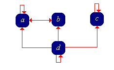
Consider a Markov chain with state space \( S = \{a, b, c, d\} \) and transition matrix \( P \) given below: \[ P = \left[ \begin{matrix} \frac{1}{3} & \frac{2}{3} & 0 & 0 \\ 1 & 0 & 0 & 0 \\ 0 & 0 & 1 & 0 \\ \frac{1}{4} & \frac{1}{4} & \frac{1}{4} & \frac{1}{4} \end{matrix} \right] \]
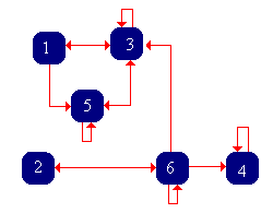
Consider a Markov chain with state space \( S = \{1, 2, 3, 4, 5, 6\} \) and transition matrix \( P \) given below: \[ P = \left[ \begin{matrix} 0 & 0 & \frac{1}{2} & 0 & \frac{1}{2} & 0 \\ 0 & 0 & 0 & 0 & 0 & 1 \\ \frac{1}{4} & 0 & \frac{1}{2} & 0 & \frac{1}{4} & 0 \\ 0 & 0 & 0 & 1 & 0 & 0 \\ 0 & 0 & \frac{1}{3} & 0 & \frac{2}{3} & 0 \\ 0 & \frac{1}{4} & \frac{1}{4} & \frac{1}{4} & 0 & \frac{1}{4} \end{matrix} \right] \]
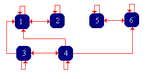
Consider a Markov chain with state space \( S = \{1, 2, 3, 4, 5, 6\} \) and transition matrix \( P \) given below: \[ P = \left[ \begin{matrix} \frac{1}{2} & \frac{1}{2} & 0 & 0 & 0 & 0 \\ \frac{1}{4} & \frac{3}{4} & 0 & 0 & 0 & 0 \\ \frac{1}{4} & 0 & \frac{1}{2} & \frac{1}{4} & 0 & 0 \\ \frac{1}{4} & 0 & \frac{1}{4} & \frac{1}{4} & 0 & \frac{1}{4} \\ 0 & 0 & 0 & 0 & \frac{1}{2} & \frac{1}{2} \\ 0 & 0 & 0 & 0 & \frac{1}{2} & \frac{1}{2} \end{matrix} \right] \]
Consider the Markov chain with state space \( S = \{1, 2, 3, 4, 5, 6, 7\} \) and transition matrix \( P \) given below:
\[ P = \left[ \begin{matrix} 0 & 0 & \frac{1}{2} & \frac{1}{4} & \frac{1}{4} & 0 & 0 \\ 0 & 0 & \frac{1}{3} & 0 & \frac{2}{3} & 0 & 0 \\ 0 & 0 & 0 & 0 & 0 & \frac{1}{3} & \frac{2}{3} \\ 0 & 0 & 0 & 0 & 0 & \frac{1}{2} & \frac{1}{2} \\ 0 & 0 & 0 & 0 & 0 & \frac{3}{4} & \frac{1}{4} \\ \frac{1}{2} & \frac{1}{2} & 0 & 0 & 0 & 0 & 0 \\ \frac{1}{4} & \frac{3}{4} & 0 & 0 & 0 & 0 & 0 \end{matrix} \right] \]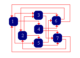
Positive recurrence, invariant distributions, and limiting distributions are discussed in separate sections for each of the following special models: