Suppose that \( G = (S, E) \) is a graph with vertex set \( S \) and edge set \( E \subseteq S^2 \). We assume that the graph is undirected (perhaps a better term would be bi-directed) in the sense that \( (x, y) \in E \) if and only if \( (y, x) \in E \). The vertex set \( S \) is countable, but may be infinite. Let \( N(x) = \{y \in S: (x, y) \in E\} \) denote the set of neighbors of a vertex \( x \in S \), and let \( d(x) = \#[N(x)] \) denote the degree of \( x \). We assume that \( N(x) \neq \emptyset \) for \( x \in S \), so \( G \) has no isolated points.
Suppose now that there is a conductance \( c(x, y) \gt 0 \) associated with each edge \( (x, y) \in E \). The conductance is symmetric in the sense that \( c(x, y) = c(y, x) \) for \( (x, y) \in E \). We extend \( c \) to a function on all of \( S \times S \) by defining \( c(x, y) = 0 \) for \( (x, y) \notin E \). Let \[ C(x) = \sum_{y \in S} c(x, y), \quad x \in S \] so that \( C(x) \) is the total conductance of the edges coming from \( x \). Our main assumption is that \( C(x) \lt \infty \) for \( x \in S \). As the terminology suggests, we imagine a fluid of some sort flowing through the edges of the graph, so that the conductance of an edge measures the capacity of the edge in some sense. One of the best interpretation is that the graph is an electrical network and the edges are resistors. In this interpretation, the conductance of a resistor is the reciprocal of the resistance.
In some applications, specifically the resistor network just mentioned, it's appropriate to impose the additional assumption that \( G \) has no loops, so that \( (x, x) \notin E \) for each \( x \in S \). However, that assumption is not mathematically necessary for the Markov chains that we will consider in this section.
The discrete-time Markov chain \( \bs{X} = (X_0, X_1, X_2, \ldots) \) with state space \( S \) and transition probability matrix \( P \) given by \[ P(x, y) = \frac{c(x, y)}{C(x)}, \quad (x, y) \in S^2 \] is called a random walk on the graph \( G \).
First, \( P(x, y) \ge 0 \) for \( x, \, y \in S \). Next, by definition of \( C \), \[ \sum_{y \in S} P(x, y) = \sum_{y \in S} \frac{c(x, y)}{C(x)} = \frac{C(x)}{C(x)} = 1, \quad x \in S \] sp \( P \) is a valid transition matrix on \( S \). Also, \( P(x, y) \gt 0 \) if and only if \( c(x, y) \gt 0 \) if and only if \( (x, y) \in E \), so the state graph of \( \bs{X} \) is \( G \), the graph we started with.
This chain governs a particle moving along the vertices of \( G \). If the particle is at vertex \( x \in S \) at a given time, then the particle will be at a neighbor of \( x \) at the next time; the neighbor is chosen randomly, in proportion to the conductance. In the setting of an electrical network, it is natural to interpret the particle as an electron. Note that multiplying the conductance function \( c \) by a positive constant has no effect on the associated random walk.
Suppose that \( d(x) \lt \infty \) for each \( x \in S \) and that \( c \) is constant on the edges. Then
The discrete-time Markov chain \( \bs{X} \) is the symmetric random walk on \( G \).
Thus, for the symmetric random walk, if the state is \( x \in S \) at a given time, then the next state is equally likely to be any of the neighbors of \( x \). The assumption that each vertex has finite degree means that the graph \( G \) is locally finite.
Let \( \bs{X} \) be a random walk on a graph \( G \).
So as usual, we will usually assume that \( G \) is connected, for otherwise we could simply restrict our attention to a component of \( G \). In the case that \( G \) has no loops (again, an important special case because of applications), it's easy to characterize the periodicity of the chain. For the theorem that follows, recall that \( G \) is bipartite if the vertex set \( S \) can be partitioned into nonempty, disjoint sets \( A \) and \( B \) (the parts) such that every edge in \( E \) has one endpoint in \( A \) and one endpoint in \( B \).
Suppose that \( \bs{X} \) is a random walk on a connected graph \( G \) with no loops. Then \( \bs{X} \) is either aperiodic or has period 2. Moreover, \( \bs{X} \) has period 2 if and only if \( G \) is bipartite, in which case the parts are the cyclic classes of \( \bs{X} \).
First note that since \( G \) is connected, the chain \( \bs{X} \) is irreducible, and so all states have the same period. If \( (x, y) \in E \) then \( (y, x) \in E \) also, so returns to \( x \in S \), starting at \( x \) can always occur at even positive integers. If \( G \) is bipartite, then returns to \( x \) starting at \( x \) can clearly only occur at even postive integers, so the period is 2. Conversely, if \( G \) is not bipartite then \( G \) has a cycle of odd length \( k \). If \( x \) is a vertex on the cycle, then returns to \( x \), starting at \( x \), can occur in 2 steps or in \( k \) steps, so the period of \( x \) is 1.
Suppose again that \( \bs{X} \) is a random walk on a graph \( G \), and assume that \( G \) is connected so that \( \bs{X} \) is irreducible.
The function \( C \) is invariant for \( P \). The random walk \( \bs{X} \) is positive recurrent if and only if \[ K = \sum_{x \in S} C(x) = \sum_{(x, y) \in S^2} c(x, y) \lt \infty \] in which case the invariant probability density function \( f \) is given by \( f(x) = C(x) / K \) for \( x \in S \).
For \( y \in S \), \[ (C P)(y) = \sum_{x \in S} C(x) P(x, y) = \sum_{x \in N(y)} C(x) \frac{c(x, y)}{C(x)} = \sum_{x \in N(y)} c(x, y) = C(y) \] so \( C \) is invariant for \( P \). The other results follow from the general theory.
Note that \( K \) is the total conductance over all edges in \( G \). In particular, of course, if \( S \) is finite then \( \bs{X} \) is positive recurrent, with \( f \) as the invariant probability density function. For the symmetric random walk, this is the only way that positive recurrence can occur:
The symmetric random walk on \( G \) is positive recurrent if and only if the set of vertices \( S \) is finite, in which case the invariant probability density function \( f \) is given by \[ f(x) = \frac{d(x)}{2 m}, \quad x \in S \] where \( d \) is the degree function and where \( m \) is the number of undirected edges.
If we take the conductance function to be the constant 1 on the edges, then \( C(x) = d(x) \) and \( K = 2 m \).
On the other hand, when \( S \) is infinite, the classification of \( \bs{X} \) as recurrent or transient is complicated. We will consider an interesting special case in for the simple random walk on \(\Z^k\).
Essentially, all reversible Markov chains can be interpreted as random walks on graphs. This fact is one of the reasons for studying such walks.
If \( \bs{X} \) is a random walk on a connected graph \( G \), then \( \bs{X} \) is reversible with respect to \( C \).
Since the graph is connected, \( \bs{X} \) is irreducible. The crucial observation is that \[ C(x) P(x, y) = C(y) P(y, x), \quad (x, y) \in S^2 \] If \( (x, y) \in E \) the left side is \( c(x, y) \) and the right side is \( c(y, x) \). If \( (x, y) \notin E \), both sides are 0. It then follows from the general theory that \( C \) is invariant for \( \bs{X} \) and that \( \bs{X} \) is reversible with respect to \( C \).
Of course, if \( \bs{X} \) is recurrent, then \( C \) is the only positive invariant function, up to multiplication by positive constants, and so \( \bs{X} \) is simply reversible.
Conversely, suppose that \( \bs{X} \) is an irreducible Markov chain on \( S \) with transition matrix \( P \) and positive invariant function \( g \). If \( \bs{X} \) is reversible with respect to \( g \) then \( \bs{X} \) is the random walk on the state graph with conductance function \( c \) given by \( c(x, y) = g(x) P(x, y) \) for \( (x, y) \in S^2 \).
Since \( \bs{X} \) is reversible with respect to \( g \), \( g \) and \( P \) satisfy \( g(x) P(x, y) = g(y) P(y, x) \) for every \( (x, y) \in S^2 \). Note that the state graph \( G \) of \( \bs{X} \) is bi-directed since \( P(x, y) \gt 0 \) if and only if \( P(y, x) \gt 0 \), and that the function \( c \) given in the theorem is symmetric, so that \( c(x, y) = c(y, x) \) for all \( (x, y) \in S^2 \). Finally, note that \[ C(x) = \sum_{y \in S} c(x, y) = \sum_{y \in S} g(x) P(x, y) = g(x), \quad x \in S \] so that \( P(x, y) = c(x, y) \big/ C(x) \) for \( (x, y) \in S^2 \), as required.
Again, in the important special case that \( \bs{X} \) is recurrent, there exists a positive invariant function \( g \) that is unique up to multiplication by positive constants. In this case the theorem states that an irreducible, recurrent, reversible chain is a random walk on the state graph.
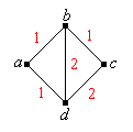
The graph below is called the Wheatstone bridge in honor of Charles Wheatstone.
In this subsection, let \( \bs{X} \) be the random walk on the Wheatstone bridge above, with the given conductance values.
For the random walk \( \bs{X} \),
For the matrix and vector below, we use the ordered state sequence \( S = (a, b, c, d) \).
For the random walk \( \bs{X} \),
For the matrix and vectors below, we use the ordered state sequence \( (a, b, c, d) \).
The graph below is the 3-dimensional cube graph. The vertices are bit strings of length 3, and two vertices are connected by an edge if and only if the bit strings differ by a single bit.
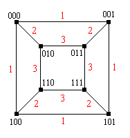
In this subsection, let \( \bs{X} \) denote the random walk on the cube graph above, with the given conductance values.
For the random walk \( \bs{X} \),
For the matrix and vector below, we use the ordered state space \( S = (000, 001, 101, 110, 010, 011, 111, 101 ) \).
For the random walk \( \bs{X} \),
For the matrix and vector below, we use the ordered state space \( S = (000, 001, 101, 110, 010, 011, 111, 101) \).
Recall that the basic Ehrenfest chain with \( m \in \N_+ \) balls is reversible. Interpreting the chain as a random walk on a graph, sketch the graph and find a conductance function.
The state graph \( G \) of the basic Ehrenfest chain with \( m \) balls is the path from 0 to \( m \) with no loops. A conductance function \( c \) is \( c(x, x + 1) = \binom{m - 1}{x} \) for \( x \in \{0, 1, \ldots, m - 1\} \).
Recall that the modified Ehrenfest chain with \( m \in \N_+ \) balls is reversible. Interpreting the chain as a random walk on a graph, sketch the graph and find a conductance function.
The state graph \( G \) of the modified Ehrenfest chain with \( m \) balls is the path from 0 to \( m \) with loops. A conductance function \( c \) is \( c(x, x + 1) = \frac{1}{2}\binom{m - 1}{x} \) for \( x \in \{0, 1, \ldots, m - 1\} \) and \( c(x, x) = \frac{1}{2} \binom{m}{x} \) for \( x \in \{0, 1, \ldots, m\} \).
Recall that the Bernoulli-Laplace chain with \( j \in \N_+ \) balls in urn 0, \( k \in \N_+\) balls in urn 1, and with \( r \in \{0, \ldots, j + k\} \) of the balls red, is reversible. Interpreting the chain as a random walk on a graph, sketch the graph and find a conductance function. Simplify the conductance function in the special case that \( j = k = r \).
The state graph \( G \) of the Bernoulli-Lapace chain with \( j \) balls in urn 0, \( k \) balls in urn 1, and with \( r \) of the balls red, is the path from \( \max\{0, r - j\} \) to \( \min\{k, r\} \) with loops. A conductance function \( c \) is given by \begin{align*} c(x, x + 1) & = \binom{r}{x} \binom{j + k - r}{k - x} (r - x)(k - x), \quad x \in \{\max\{0, r - j\}, \ldots, \min\{k, r\} - 1\} \\ c(x, x) & = \binom{r}{x} \binom{j + k - r}{k - x} [(r - x) x + (j - r + x)(k - x)], \quad x \in \{\max\{0, r - j\}, \ldots, \min\{k, r\}\} \end{align*} In the special case that \( j = k = r \), a conductance function is \begin{align*} c(x, x + 1) & = \binom{k}{x} \binom{k}{k - x} (k - x)^2, \quad x \in \{0, \ldots, k - 1\} \\ c(x, x) & = \binom{k}{x} \binom{k}{k - x} 2 x (k - x), \quad x \in \{0, \ldots, k\} \end{align*}
Random walks on integer lattices are particularly interesting because of their classification as transient or recurrent. We consider the one-dimensional case in this subsection, and the higher dimensional case in the next subsection.
Let \( \bs{X} = (X_0, X_1, X_2, \ldots) \) be the discrete-time Markov chain with state space \( \Z \) and transition probability matrix \( P \) given by \[ P(x, x + 1) = p, \; P(x, x - 1) = 1 - p, \quad x \in \Z \] where \( p \in (0, 1) \). The chain \( \bs{X} \) is called the simple random walk on \( \Z \) with parameter \( p \).
The term simple is used because the transition probabilities starting in state \( x \in \Z \) do not depend on \( x \). Thus the chain is spatially as well as temporally homogeneous. In the special case \( p = \frac{1}{2} \), the chain \( \bs{X} \) is the simple symmetric random walk on \( \Z \). Basic properties of the simple random walk on \( \Z \), and in particular, the simple symmetric random walk were studied in Chapter 10 on Bernoulli trials. Of course, the state graph \( G \) of \( \bs{X} \) has vertex set \( \Z \), and the neighbors of \( x \in \Z \) are \( x + 1 \) and \( x - 1 \). It's not immediately clear that \( \bs{X} \) is a random walk on \( G \) associated with a conductance function, which after all, is the topic of this section. But that fact and more follow from the next result.
Let \( g \) be the function on \( \Z \) defined by \[ g(x) = \left(\frac{p}{1 - p}\right)^x, \quad x \in \Z \] Then
In particular, the simple symmetric random walk is the symmetric random walk on \( G \).
The chain \( \bs{X} \) is irreducible and periodic with period 2. Moreover \[ P^{2 n}(0, 0) = \binom{2 n}{n} p^n (1 - p)^n, \quad n \in \N \]
The chain is irreducible since \( G \) is connected. The chain is periodic since \( G \) has no loops and is bipartite, with the parts being the odd and even integers. Finally, note that starting in state 0, the chain returns to 0 at time \( 2 n \) if and only if there are \( n \) steps to the right and \( n \) steps to the left.
Classification of the simple random walk on \( \Z \).
From and Stirling's approximation, \[ P^{2 n}(0, 0) \approx \frac{[4 p (1 - p)]^n}{\sqrt{\pi \, n}} \text{ as } n \to \infty \] Let \( R(x, y) = \sum_{n=0}^\infty P^n(x, y) \) for \( (x, y) \in \Z^2 \), so that \(R\) is the potential matrix. Recall that \( R(x, y) \) is the expected number of visits to \( y \) starting in \( x \) for \( (x, y) \in \Z^2 \). If \( p \ne \frac{1}{2} \) then \( R(0, 0) \lt \infty \) and hence \( \bs{X} \) is transient. If \( p = \frac{1}{2} \) then \( R(0, 0) = \infty \) and hence \( \bs{X} \) is recurrent. In this case \( \bs{X} \) must be null recurrent from exercuse , since the vertex set is infinite.
So for the one-dimensional lattice \( \Z \), the random walk \( \bs{X} \) is transient in the non-symmetric case, and null recurrent in the symmetric case. Let's return to the invariant functions of \( \bs{X} \)
Consider again the random walk \( \bs{X} \) on \( \Z \) with parameter \( p \in (0, 1) \). The constant function \(\bs{1} \) on \( \Z \) and the function \( g\) given by \[ g(x) = \left(\frac{p}{1 - p}\right)^x, \quad x \in \Z \] are invariant for \( \bs{X} \). All other invariant functions are linear combinations of these two functions.
The condition for \( h \) to be invariant, \( h P = h \), leads to the following linear, second order difference equation: \[(1 - p) h(y + 1) - h(y) + (1 + p) h(y - 1), \quad y \in \Z\] The characteristic equation is \( (1 - p) r^2 - r + (1 + p) = 0 \) which has roots \( r = 1 \) and \( r = p \big/ (1 - p) \). The solutions corresponding to the roots are \( \bs{1} \) and \( g \), respectively. Hence the result follows from the general theory of linear difference equations.
Note that when \( p = \frac{1}{2} \), the constant function \( \bs{1} \) is the only positive invariant function, up to multiplication by positive constants. But we know this has to be the case since the chain is recurrent when \( p = \frac{1}{2} \). Moreover, the chain is reversible. In the non-symmetric case, when \( p \ne \frac{1}{2} \), we have an example of a transient chain which nonetheless has non-trivial invariant functions—in fact a two dimensional space of such functions. Also, \( \bs{X} \) is reversible with respect to \( g \), as shown in , but the reversal of \( \bs{X} \) with respect to \( \bs{1} \) is the chain with transition matrix \( Q \) given by \( Q(x, y) = P(y, x) \) for \( (x, y) \in \Z^2 \). This chain is just the simple random walk on \( Z \) with parameter \( 1 - p \). So the non-symmetric simple random walk is an example of a transient chain that is reversible with respect to one invariant measure but not with respect to another invariant measure.
More generally, we now consider \( \Z^k \), where \( k \in \N_+ \). For \( i \in \{1, 2, \ldots, k\} \), let \( \bs{u}_i \in \Z^k \) denote the unit vector with 1 in position \( i \) and 0 elsewhere. The \( k \)-dimensional integer lattice \( G \) has vertex set \( Z^k \), and the neighbors of \( \bs{x} \in \Z^k \) are \( \bs{x} \pm \bs{u}_i \) for \( i \in \{1, 2, \ldots, k\} \). So in particular, each vertex has \( 2 k \) neighbors.
Let \( \mathscr{X} = (\bs{X}_1, \bs{X_2}, \ldots) \) be the Markov chain on \( \Z^k \) with transition probability matrix \( P \) given by \[ P(\bs{x},\bs{x} + \bs{u}_i) = p_i, \; P(\bs{x}, \bs{x} - \bs{u}_i) = q_i; \quad \bs{x} \in \Z^k, \; i \in \{1, 2, \ldots, k\} \] where \( p_i \gt 0 \), \( q_i \gt 0 \) for \( i \in \{1, 2, \ldots, k\} \) and \( \sum_{i=1}^k (p_i + q_i) = 1 \). The chain \( \mathscr{X} \) is the simple random walk on \( \Z^k \) with parameters \( \bs{p} = (p_1, p_2, \ldots, p_k) \) and \( \bs{q} = (q_1, q_2, \ldots, q_k) \).
Again, the term simple means that the transition probabilities starting at \( \bs{x} \in \Z^k \) do not depend on \( \bs{x} \), so that the chain is spatially homogeneous as well as temporally homogeneous. In the special case that \( p_i = q_i = \frac{1}{2 k} \) for \( i \in \{1, 2, \ldots, k\} \), \( \mathscr{X} \) is the simple symmetric random walk on \( Z^k \). The following theorem is the natural generalization of in the one-dimensional case.
Define the function \( g: \Z^k \to (0, \infty) \) by \[ g(x_1, x_2, \ldots, x_k) = \prod_{i=1}^k \left(\frac{p_i}{q_i}\right)^{x_i}, \quad (x_1, x_2, \ldots, x_k) \in \Z^k \] Then
Classification of the simple random walk on \( \Z^k \).
For certain of the non-symmetric cases, we can use the result for dimension 1. Suppose \( i \in \{1, 2, \ldots, k\} \) with \( p_i \ne q_i \). If we consider the times when coordinate \( i \) of the random walk \( \mathscr{X} \) changes, we have an embedded one-dimensional random walk with parameter \( p = p_i \big/ (p_i + q_i) \) (the probability of a step in the positive direction). Since \( p \ne \frac{1}{2} \), this embedded random walk is transient and so will fail to return to 0, starting at 0, with positive probability. But if this embedded random walk fails to return to 0, starting at 0, then the parent random walk \( \mathscr{X} \) fails to return to \( \bs{0} \) starting at \( \bs{0} \). Hence \( \mathscr{X} \) is transient.
For the symmetric case, the general proof is similar in to the proof for dimension 1 in , but the details are considerably more complex. A return to \( 0 \) can occur only at even times and \[ P^{2 n}(\bs{0}, \bs{0}) \approx \frac{C_k}{n^{k/2}} \text{ as } n \to \infty \text{ where } C_k = \frac{k^{k/2}}{\pi^{k/2} 2^{k-1}}\] Thus for the potential matrix \( R \) we have \( R(\bs{0}, \bs{0}) = \infty \) and the chain is recurrent if \( k \in \{1, 2\} \) while \( R(\bs{0}, \bs{0}) \lt \infty \) and the chain is transient if \( k \in \{3, 4, \ldots\} \).
So for the simple, symmetric random walk on the integer lattice \( \Z^k \), we have the following interesting dimensional phase shift: the chain is null recurrent in dimensions 1 and 2 and transient in dimensions 3 or more.
Let's return to the positive invariant functions for \( \mathscr{X} \). Again, the results generalize those for the one-dimensional case.
For \( J \subseteq \{1, 2 \ldots, k\} \), define \( g_J \) on \( \Z^k \) by \[ g_J(x_1, x_2, \ldots, x_k) = \prod_{j \in J} \left(\frac{p_j}{q_j}\right)^{x_j}, \quad (x_1, x_2, \ldots, x_k) \in \Z^k \] Let \( \mathscr{X}_J \) denote the simple random walk on \( \Z^k \) with transition matrix \( P_J \), corresponding to the parameter vectors \( \bs{p}^J \) and \( \bs{q^J} \), wherre \(p^J_j = p_j \), \(q^J_j = q_j \) for \( j \in J \), and \( p^J_j = q_j \), \(q^J_j = p_j \) for \( j \notin J \). Then
Part (a) follows from simple substitution. Parts (b) and (c) follow from (a) and the general theory.
Note that when \( J = \emptyset \), \( g_J = \bs{1} \) and when \( J = \{1, 2, \ldots, k\} \), \( g_J = g \), the invariant function introduced in . So in the completely non-symmetric case where \( p_i \ne q_i \) for every \( i \in \{1, 2, \ldots, k\} \), the random walk \( \mathscr{X} \) has \( 2^k \) positive invariant functions that are linearly independent, and \( \mathscr{X} \) is reversible with respect to one of them.