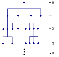
Generically, suppose that we have a system of particles that can generate or split into other particles of the same type. Here are some typical examples:
We assume that each particle, at the end of its life, is replaced by a random number of new particles that we will refer to as children of the original particle. Our basic assumption is that the particles act independently, each with the same offspring distribution on \( \N \). Let \( f \) denote the common probability density function of the number of offspring of a particle. We will also let \( f^{*n} = f * f * \cdots * f \) denote the convolution power of degree \( n \) of \( f \); this is the probability density function of the total number of children of \( n \) particles.
We will consider the evolution of the system in real time in our study of continuous-time branching chains. In this section, we will study the evolution of the system in generational time. Specifically, the particles that we start with are in generation 0, and recursively, the children of a particle in generation \( n \) are in generation \( n + 1 \).
Let \( X_n \) denote the number of particles in generation \( n \in \N \). One way to construct the process mathematically is to start with an array of independent random variables \( (U_{n,i}: n \in \N, \; i \in \N_+) \), each with probability density function \( f \). We interpret \( U_{n,i} \) as the number of children of the \( i \)th particle in generation \( n \) (if this particle exists). Note that we have more random variables than we need, but this causes no harm, and we know that we can construct a probability space that supports such an array of random variables. We can now define our state variables recursively by \[ X_{n+1} = \sum_{i=1}^{X_n} U_{n,i} \]
\( \bs{X} = (X_0, X_1, X_2, \ldots) \) is a discrete-time Markov chain on \( \N \) with transition probability matrix \( P \) given by \[ P(x, y) = f^{*x}(y), \quad (x, y) \in \N^2 \] The chain \( \bs{X} \) is the branching chain with offspring distribution defined by \( f \).
The Markov property and the form of the transition matrix follow directly from the construction of the state variables given above. Since the variables \( (U_{n,i}: n \in \N, i \in \N_+) \) are independent, each with PDF \( f \), we have \[ \P(X_{n+1} = y \mid X_0 = x_0, \ldots, X_{n-1} = x_{n-1}, X_n = x) = \P\left(\sum_{i=1}^x U_{n,i} = y\right) = f^{*x}(y) \]
The branching chain is also known as the Galton-Watson process in honor of Francis Galton and Henry William Watson who studied such processes in the context of the survival of (aristocratic) family names. Note that the descendants of each initial particle form a branching chain, and these chains are independent. Thus, the branching chain starting with \( x \) particles is equivalent to \( x \) independent copies of the branching chain starting with 1 particle. This features turns out to be very important in the analysis of the chain. Note also that 0 is an absorbing state that corresponds to extinction. On the other hand, the population may grow to infinity, sometimes called explosion. Computing the probability of extinction is one of the fundamental problems in branching chains; we will essentially solve this problem in the next subsection.
The behavior of the branching chain in expected value) is easy to analyze. Let \( m \) denote the mean of the offspring distribution, so that \[ m = \sum_{x=0}^\infty x f(x) \] Note that \( m \in [0, \infty] \). The parameter \( m \) will turn out to be of fundamental importance.
Expected value properties
For part (a) we use a conditioning argument and the construction above. For \( x \in \N \), \[ \E(X_{n+1} \mid X_n = x) = \E\left(\sum_{i=1}^x U_{n,i} \biggm| X_n = x\right) = \E\left(\sum_{i=1}^x U_{n,i}\right) = m x \] That is, \( \E(X_{n+1} \mid X_n) = m X_n \) so \( \E(X_{n+1}) = \E\left[\E(X_{n+1} \mid X_n)\right] = m \E(X_n) \) Part (b) follows from (a) and then parts (c), (d), and (e) follow from (b).
Part (c) of is extinction in the mean; part (d) is stability in the mean; and part (e) is explosion in the mean.
Recall that state 0 is absorbing (there are no particles), and hence \( \{X_n = 0 \text{ for some } n \in \N\} = \{\tau_0 \lt \infty\} \) is the extinction event (where as usual, \( \tau_0 \) is the time of the first return to 0). We are primarily concerned with the probability of extinction, as a function of the initial state. First, however, we will make some simple observations and eliminate some trivial cases.
Suppose that \( f(1) = 1 \), so that each particle is replaced by a single new particle. Then
These properties are obvious since \( P(x, x) = 1 \) for every \( x \in \N \).
Suppose that \( f(0) \gt 0 \) so that with positive probability, a particle will die without offspring. Then
Suppose that \( f(0) = 0 \) and \( f(1) \lt 1 \), so that every particle is replaced by at least one particle, and with positive probability, more than one. Then
Suppose that \( f(0) \gt 0 \) and \( f(0) + f(1) = 1 \), so that with positive probability, a particle will die without offspring, and with probability 1, a particle is not replaced by more than one particle. Then
Thus, the interesting case is when \( f(0) \gt 0 \) and \( f(0) + f(1) \lt 1 \), so that with positive probability, a particle will die without offspring, and also with positive probability, the particle will be replaced by more than one new particles. We will assume these conditions for the remainder of our discussion. By , all states lead to 0 (extinction). We will denote the probability of extinction, starting with one particle, by \[ q = \P(\tau_0 \lt \infty \mid X_0 = 1) = \P(X_n = 0 \text{ for some } n \in \N \mid X_0 = 1) \]
The set of positive states \( \N_+ \) is a transient equivalence class, and the probability of extinction starting with \( x \in \N \) particles is \[ q^x = \P(\tau_0 \lt \infty \mid X_0 = x) = \P(X_n = 0 \text{ for some } n \in \N \mid X_0 = x) \]
Under the assumptions on \( f \), from any positive state the chain can move 2 or more units to the right and one unit to the left in one step. It follows that every positive state leads to every other positive state. On the other hand, every positive state leads to 0, which is absorbing. Thus, \( \N_+ \) is a transient equivalence class.
Recall that the branching chain starting with \( x \in \N_+ \) particles acts like \( x \) independent branching chains starting with one particle. Thus, the extinction probability starting with \( x \) particles is \( q^x \).
The parameter \( q \) satisfies the equation \[ q = \sum_{x = 0}^\infty f(x) q^x \]
This result follows from conditioning on the first state. \[ q = \P(\tau_0 \lt \infty \mid X_0 = 1) = \sum_{x = 0}^\infty \P(\tau_0 \lt \infty \mid X_0 = 1, X_1 = x) \P(X_1 = x \mid X_0 = 1) \] But by the Markov property and the previous result, \[ \P(\tau_0 \lt \infty \mid X_0 = 1, X_1 = x) = \P(\tau_0 \lt \infty \mid X_1 = x) = q^x \] and of course \( \P(X_1 = x \mid X_0 = 1) = P(1, x) = f(x) \).
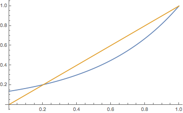
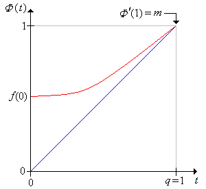
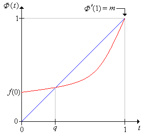
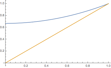
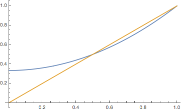
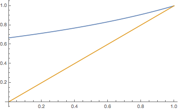
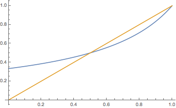
Thus the extinction probability \( q \) starting with 1 particle is a fixed point of the probability generating function \( \Phi \) of the offspring distribution: \[ \Phi(t) = \sum_{x=0}^\infty f(x) t^x, \quad t \in [0, 1] \] Moreover, from the general discussion of hitting probabilities in the section on recurrence and transience, \( q \) is the smallest such number in the interval \( (0, 1] \). If the probability generating function \( \Phi \) can be computed in closed form, then \( q \) can sometimes be computed by solving the equation \( \Phi(t) = t \).
\( \Phi \) satisfies the following properties:
These are basic properties of the probability generating function. Recall that the series that defines \( \Phi \) is a power series about 0 with radius of convergence \( r \ge 1 \). A function defined by a power series is infinitely differentiable within the open interval of convergence, and the derivates can be computed term by term. So \begin{align*} \Phi^\prime(t) &= \sum_{x=1}^\infty x f(x) t^{x-1} \gt 0, \quad t \in (0, 1) \\ \Phi^{\prime \prime}(t) &= \sum_{x=2}^\infty x (x - 1) f(x) t^{x - 2} \gt 0, \quad t \in (0, 1) \end{align*} If \( r \gt 1 \) then \( m = \Phi^\prime(1) \). If \( r = 1 \), the limit result is the best we can do.
Our main result is next, and relates the extinction probability \( q \) and the mean of the offspring distribution \( m \).
The extinction probability \( q \) and the mean of the offspring distribution \( m \) are related as follows:
These results follow from the properties of the PGF \( \Phi \) in . See the graphs below.
Consider the branching chain with offspring probability density function \( f \) given by \( f(0) = 1 - p \), \( f(2) = p \), where \( p \in (0, 1) \) is a parameter. Thus, each particle either dies or splits into two new particles. Find each of the following.
Note that an offspring variable has the form \( 2 I \) where \( I \) is an indicator variable with parameter \( p \).
Consider the branching chain whose offspring distribution is the geometric distribution on \( \N \) with parameter \( 1 - p \), where \( p \in (0, 1) \). Thus \( f(n) = (1 - p) p^n \) for \( n \in \N \). Find each of the following:
Curiously, the extinction probability is the same as in .
Consider the branching chain whose offspring distribution is the Poisson distribution with parameter \( m \in (0, \infty) \). Thus \( f(n) = e^{-m} m^n / n! \) for \( n \in \N \). Find each of the following: