

In this section we will study an interesting problem known variously as the secretary problem or the marriage problem. It is simple to state and not difficult to solve, but the solution is a bit surprising. Also, the problem serves as a nice introduction to the general area of statistical decision making.
As always, we must start with a clear statement of the problem.
We have \(n\) candidates (perhaps applicants for a job or possible marriage partners). The assumptions are
The assumptions, of course, are not entirely reasonable in real applications. The last assumption, for example, that \(n\) is known, is more appropriate for the secretary interpretation than for the marriage interpretation.
What is an optimal strategy? What is the probability of success with this strategy? What happens to the strategy and the probability of success as \(n\) increases? In particular, when \(n\) is large, is there any reasonable hope of finding the best candidate?
Play the secretary game several times with \(n = 10\) candidates. See if you can find a good strategy just by trial and error.
After playing the secretary game a few times, it should be clear that the only reasonable type of strategy is to let a certain number \(k - 1\) of the candidates go by, and then select the first candidate we see who is better than all of the previous candidates (if she exists). If she does not exist (that is, if no candidate better than all previous candidates appears), we will agree to accept the last candidate, even though this means failure. The parameter \(k\) must be between 1 and \(n\); if \(k = 1\), we select the first candidate; if \(k = n\), we select the last candidate; for any other value of \(k\), the selected candidate is random, distributed on \(\{k, k + 1, \ldots, n\}\). We will refer to this let \(k - 1\) go by
strategy as strategy \(k\).
Thus, we need to compute the probability of success \(p_n(k)\) using strategy \(k\) with \(n\) candidates. Then we can maximize the probability over \(k\) to find the optimal strategy, and then take the limit over \(n\) to study the asymptotic behavior.
First, let's do some basic computations.
For the case \(n = 3\), list the 6 permutations of \(\{1, 2, 3\}\) and verify the probabilities in the table below. Note that \(k = 2\) is optimal.
| \(k\) | 1 | 2 | 3 |
|---|---|---|---|
| \(p_3(k)\) | \(\frac{2}{6}\) | \(\frac{3}{6}\) | \(\frac{2}{6}\) |
The following table gives the \( 3! = 6 \) permutations of the candidates \( (1, 2, 3) \), and the candidate selected by each strategy. The last row gives the total number of successes for each strategy.
| Permutation | \(k = 1\) | \(k = 2\) | \(k = 3\) |
|---|---|---|---|
| \((1, 2, 3)\) | 1 | 3 | 3 |
| \((1, 3, 2)\) | 1 | 2 | 2 |
| \((2, 1, 3)\) | 2 | 1 | 3 |
| \((2, 3, 1)\) | 2 | 1 | 1 |
| \((3, 1, 2)\) | 3 | 1 | 2 |
| \((3, 2, 1)\) | 3 | 2 | 1 |
| Total | 2 | 3 | 2 |
In the secretary experiment, set the number of candidates to \(n = 3\). Run the experiment 1000 times with each strategy \( k \in \{1, 2, 3\} \)
For the case \(n = 4\), list the 24 permutations of \(\{1, 2, 3, 4\}\) and verify the probabilities in the table below. Note that \(k = 2\) is optimal. The last row gives the total number of successes for each strategy.
| \(k\) | 1 | 2 | 3 | 4 |
|---|---|---|---|---|
| \(p_4(k)\) | \(\frac{6}{24}\) | \(\frac{11}{24}\) | \(\frac{10}{24}\) | \(\frac{6}{24}\) |
The following table gives the \(4! = 24\) permutations of the candidates \((1, 2, 3, 4)\), and the candidate selected by each strategy.
| Permutation | \(k = 1\) | \(k = 2\) | \(k = 3\) | \(k = 4\) |
|---|---|---|---|---|
| \((1, 2, 3, 4)\) | 1 | 4 | 4 | 4 |
| \((1, 2, 4, 3)\) | 1 | 3 | 3 | 3 |
| \((1, 3, 2, 4)\) | 1 | 4 | 4 | 4 |
| \((1, 3, 4, 2)\) | 1 | 3 | 2 | 2 |
| \((1, 4, 2, 3)\) | 1 | 3 | 3 | 3 |
| \((1, 4, 3, 2)\) | 1 | 2 | 2 | 2 |
| \((2, 1, 3, 4)\) | 2 | 1 | 4 | 4 |
| \((2, 1, 4, 3)\) | 2 | 1 | 3 | 3 |
| \((2, 3, 1, 4)\) | 2 | 1 | 1 | 4 |
| \((2, 3, 4, 1)\) | 2 | 1 | 1 | 1 |
| \((2, 4, 1, 3)\) | 2 | 1 | 1 | 3 |
| \((2, 4, 3, 1)\) | 2 | 1 | 1 | 1 |
| \((3, 1, 2, 4)\) | 3 | 1 | 4 | 4 |
| \((3, 1, 4, 2)\) | 3 | 1 | 2 | 2 |
| \((3, 2, 1, 4)\) | 3 | 2 | 1 | 4 |
| \((3, 2, 4, 1)\) | 3 | 2 | 1 | 1 |
| \((3, 4, 1, 2)\) | 3 | 1 | 1 | 2 |
| \((3, 4, 2, 1)\) | 3 | 2 | 2 | 1 |
| \((4, 1, 2, 3)\) | 4 | 1 | 3 | 3 |
| \((4, 1, 3, 2)\) | 4 | 1 | 2 | 2 |
| \((4, 2, 1, 3)\) | 4 | 2 | 1 | 3 |
| \((4, 2, 3, 1)\) | 4 | 2 | 1 | 1 |
| \((4, 3, 1, 2)\) | 4 | 3 | 1 | 2 |
| \((4, 3, 2, 1)\) | 4 | 3 | 2 | 1 |
| Total | 6 | 11 | 10 | 6 |
In the secretary experiment, set the number of candidates to \(n = 4\). Run the experiment 1000 times with each strategy \( k \in \{1, 2, 3, 4\} \)
For the case \(n = 5\), list the 120 permutations of \(\{1, 2, 3, 4, 5\}\) and verify the probabilities in the table below. Note that \(k = 3\) is optimal.
| \(k\) | 1 | 2 | 3 | 4 | 5 |
|---|---|---|---|---|---|
| \(p_5(k)\) | \(\frac{24}{120}\) | \(\frac{50}{120}\) | \(\frac{52}{120}\) | \(\frac{42}{120}\) | \(\frac{24}{120}\) |
In the secretary experiment, set the number of candidates to \(n = 5\). Run the experiment 1000 times with each strategy \( k \in \{1, 2, 3, 4, 5\} \)
Well, clearly we don't want to keep doing this. Let's see if we can find a general analysis. With \(n\) candidates, let \(X_n\) denote the number (arrival order) of the best candidate, and let \(S_{n,k}\) denote the event of success for strategy \(k\) (we select the best candidate).
\(X_n\) is uniformly distributed on \(\{1, 2, \ldots, n\}\).
This follows since the candidates arrive in random order.
Next we will compute the conditional probability of success given the arrival order of the best candidate.
For \( n \in \N_+ \) and \( k \in \{2, 3, \ldots, n\} \), \[ \P(S_{n,k} \mid X_n = j) = \begin{cases} 0, & j \in \{1, 2, \ldots, k-1\} \\ \frac{k-1}{j-1}, & j \in \{k, k + 1, \ldots, n\} \end{cases} \]
For the first case, note that if the arrival number of the best candidate is \(j \lt k\), then strategy \(k\) will certainly fail. For the second cases, note that if the arrival order of the best candidate is \(j \ge k\), then strategy \(k\) will succeed if and only if one of the first \(k - 1\) candidates (the ones that are automatically rejected) is the best among the first \(j - 1\)
The two cases are illustrated below. The large dot indicates the best candidate. Red dots indicate candidates that are rejected out of hand, while blue dots indicate candidates that are considered.


Now we can compute the probability of success with strategy \(k\).
For \( n \in \N_+ \) \[ p_n(k) = \P(S_{n,k}) = \begin{cases} \frac{1}{n}, & k = 1 \\ \frac{k - 1}{n} \sum_{j=k}^n \frac{1}{j - 1}, & k \in \{2, 3, \ldots, n\} \end{cases} \]
When \( k = 1 \) we simply select the first candidate. This candidate will be the best one with probability \( 1 / n \). The result for \( k \in \{2, 3, \ldots, n\} \) follows from and , by conditioning on \(X_n\): \[ \P(S_{n,k}) = \sum_{j=1}^n \P(X_n = j) \P(S_{n,k} \mid X_n = j) = \sum_{j=k}^n \frac{1}{n} \frac{k - 1}{j - 1} \]
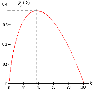
Values of the function \(p_n\) can be computed by hand for small \(n\) and by a computer algebra system for moderate \(n\). The graph of \(p_{100}\) is shown below. Note the concave downward shape of the graph and the optimal value of \(k\), which turns out to be 38. The optimal probability is about 0.37104.
The optimal strategy \(k_n\) that maximizes \(k \mapsto p_n(k)\), the ratio \(k_n / n\), and the optimal probability \(p_n(k_n)\) of finding the best candidate, as functions of \(n \in \{3, 4, \dots, 20\}\) are given in the following table:
| Candidates \(n\) | Optimal strategy \(k_n\) | Ratio \(k_n / n\) | Optimal probability \(p_n(k_n)\) |
|---|---|---|---|
| 3 | 2 | 0.6667 | 0.5000 |
| 4 | 2 | 0.5000 | 0.4583 |
| 5 | 3 | 0.6000 | 0.4333 |
| 6 | 3 | 0.5000 | 0.4278 |
| 7 | 3 | 0.4286 | 0.4143 |
| 8 | 4 | 0.5000 | 0.4098 |
| 9 | 4 | 0.4444 | 0.4060 |
| 10 | 4 | 0.4000 | 0.3987 |
| 11 | 5 | 0.4545 | 0.3984 |
| 12 | 5 | 0.4167 | 0.3955 |
| 13 | 6 | 0.4615 | 0.3923 |
| 14 | 6 | 0.4286 | 0.3917 |
| 15 | 6 | 0.4000 | 0.3894 |
| 16 | 7 | 0.4375 | 0.3881 |
| 17 | 7 | 0.4118 | 0.3873 |
| 18 | 7 | 0.3889 | 0.3854 |
| 19 | 8 | 0.4211 | 0.3850 |
| 20 | 8 | 0.4000 | 0.3842 |
Apparently, as we might expect, the optimal strategy \(k_n\) increases and the optimal probability \(p_n(k_n)\) decreases as \(n \to \infty\). On the other hand, it's encouraging, and a bit surprising, that the optimal probability does not appear to be decreasing to 0. It's perhaps least clear what's going on with the ratio. Graphical displays of some of the information in the table may help:
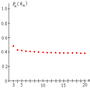
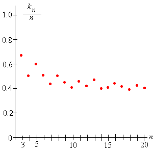
Could it be that the ratio \(k_n / n\) and the probability \(p_n(k_n)\) are both converging, and moreover, are converging to the same number? First let's try to establish rigorously some of the trends observed in the table.
The success probability \(p_n\) satisfies \[ p_n(k - 1) \lt p_n(k) \text{ if and only if } \sum_{j=k}^n \frac{1}{j-1} \gt 1 \]
It follows that for each \(n \in \N_+\), the function \(p_n\) at first increases and then decreases. The maximum value of \(p_n\) occurs at the largest \(k\) with \(\sum_{j=k}^n \frac{1}{j - 1} \gt 1\). This is the optimal strategy with \(n\) candidates, which we have denoted by \(k_n\).
As \(n\) increases, \(k_n\) increases and the optimal probability \(p_n(k_n)\) decreases.
We are naturally interested in the asymptotic behavior of the function \(p_n\), and the optimal strategy as \(n \to \infty\). The key is recognizing \(p_n\) as a Riemann sum for a simple integral. (Riemann sums, of course, are named for Georg Riemann.)
If \(k(n)\) depends on \(n\) and \(k(n) / n \to x \in (0, 1)\) as \(n \to \infty\) then \(p_n[k(n)] \to -x \ln x\) as \(n \to \infty\).
First note that \[ p_n(k) = \frac{k-1}{n} \sum_{j=k}^n \frac{1}{n} \frac{n}{j-1} \] We recognize the sum above as the left Riemann sum for the the function \(f(t) = \frac{1}{t}\) corresponding to the partition of the interval \(\left[\frac{k-1}{n}, 1\right]\) into \((n - k) + 1\) subintervals of length \(\frac{1}{n}\) each: \(\left(\frac{k-1}{n}, \frac{k}{n}, \ldots, \frac{n-1}{n}, 1\right)\). It follows that \[ p_n[k(n)] \to x \int_x^1 \frac{1}{t} dt = -x \ln x \text{ as } n \to \infty\]
The optimal strategy \(k_n\) that maximizes \(k \mapsto p_n(k)\), the ratio \(k_n / n\), and the optimal probability \(p_n(k_n)\) of finding the best candidate, as functions of \(n \in \{10, 20, \dots, 100\}\) are given in the following table:
| Candidates \(n\) | Optimal strategy \(k_n\) | Ratio \(k_n / n\) | Optimal probability \(p_n(k_n)\) |
|---|---|---|---|
| 10 | 4 | 0.4000 | 0.3987 |
| 20 | 8 | 0.4000 | 0.3842 |
| 30 | 12 | 0.4000 | 0.3786 |
| 40 | 16 | 0.4000 | 0.3757 |
| 50 | 19 | 0.3800 | 0.3743 |
| 60 | 23 | 0.3833 | 0.3732 |
| 70 | 27 | 0.3857 | 0.3724 |
| 80 | 30 | 0.3750 | 0.3719 |
| 90 | 34 | 0.3778 | 0.3714 |
| 100 | 38 | 0.3800 | 0.3710 |
The graph below shows the true probabilities \(p_n(k)\) and the limiting values \(-\frac{k}{n} \, \ln\left(\frac{k}{n}\right)\) as a function of \(k\) with \(n = 100\).
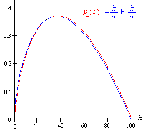
For the optimal strategy \(k_n\), there exists \(x_0 \in (0, 1)\) such that \(k_n / n \to x_0\) as \(n \to \infty\). Thus, \(x_0 \in (0, 1)\) is the limiting proportion of the candidates that we reject out of hand. Moreover, \(x_0\) maximizes \(x \mapsto -x \ln x\) on \((0, 1)\).
The maximum value of \(-x \ln x\) occurs at \(x_0 = 1 / e\) and the maximum value is also \(1 / e\).
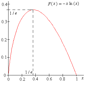
The special number \(1 / e \approx 0.3679\) occurs twice in the problem. For large \(n\):
The article Who Solved the Secretary Problem?
by Tom Ferguson (1989) has an interesting historical discussion of the problem, including speculation that Johannes Kepler may have used the optimal strategy to choose his second wife. The article also discusses many interesting generalizations of the problem. A different version of the secretary problem, in which the candidates are assigned a score in \([0, 1]\), rather than a relative rank, is discussed in the section on stopping times in the chapter on martingales