As the name suggests, the log-logistic distribution is the distribution of a variable whose logarithm has the logistic distribution. The log-logistic distribution is often used to model random lifetimes, and hence has applications in reliability.
The basic log-logistic distribution with shape parameter \( k \in (0, \infty) \) is a continuous distribution on \( [0, \infty) \) with distribution function \( G \) given by \[ G(z) = \frac{z^k}{1 + z^k}, \quad z \in [0, \infty) \] In the special case that \( k = 1 \), the distribution is the standard log-logistic distribution.
Note that \( G \) is continuous on \( [0, \infty) \) with \( G(0) = 0 \) and \( G(z) \to 1 \) as \( z \to \infty \). Moreover, \[ g(z) = G^\prime(z) = \frac{k z^{k-1}}{(1 + z^k)^2} \gt 0, \quad z \in (0, \infty) \] so \( G \) is strictly increasing on \( [0, \infty) \).
The probability density function function \( g \) is given by \[ g(z) = \frac{k z^{k-1}}{(1 + z^k)^2}, \quad z \in (0, \infty) \]
The PDF \( g = G^\prime \) was computed in the details of . The rest follows from calculus: \begin{align} g^{\prime}(z) & = \frac{k z^{k-2}[(k - 1) - (k + 1) z^k]}{(1 + z^k)^3}, \quad z \in (0, \infty) \\ g^{\prime \prime}(z) & = \frac{k z^{k - 3} \left[(k - 1)(k - 2) - 4(k^2 -1) z^k + (k + 1) (k + 2)z^{2 k}\right]}{(1 + z^k)^4}, \quad z \in (0, \infty) \end{align}
So \( g \) has a rich variety of shapes, and is unimodal if \( k \gt 1 \). When \( k \ge 1 \), \( g \) is defined at 0 as well.
Open the special distribution simulator and select the log-logistic distribution. Vary the shape parameter and note the shape of the probability density function. For selected values of the shape parameter, run the simulation 1000 times and compare the empirical density function to the probability density function.
The quantile function \( G^{-1} \) is given by \[ G^{-1}(p) = \left(\frac{p}{1 - p}\right)^{1/k}, \quad p \in [0, 1) \]
Recall that \( p \big/ (1 - p) \) is the odds ratio associated with probability \( p \in (0, 1) \). Thus, the quantile function of the basic log-logistic distribution with shape parameter \( k \) is the \( k \)th root of the odds ratio. In particular, the quantile function of the standard log-logistic distribution is the odds ratio itself. Also of interest is that the median is 1 for every value of the shape parameter.
Open the quantile app and select the log-logistic distribution. Vary the shape parameter and note the shape of the distribution and probability density functions. For selected values of the shape parameter, compute the quantiles of order 0.1 and 0.9.
The reliability function \( G^c \) is given by \[ G^c(z) = \frac{1}{1 + z^k}, \quad z \in [0, \infty) \]
The basic log-logistic distribution has either decreasing failure rate, or mixed decreasing-increasing failure rate, depending on the shape parameter.
The failure rate function \( r \) is given by \[ r(z) = \frac{k z^{k-1}}{1 + z^k}, \quad z \in (0, \infty) \]
If \( k \ge 1 \), \( r \) is defined at 0 also.
Suppose that \( Z \) has the basic log-logistic distribution with shape parameter \( k \in (0, \infty) \). The moments (about 0) of the \( Z \) have an interesting expression in terms of the beta function \( B \) and in terms of the sine function. The simplest representation is in terms of a new special function constructed from the sine function.
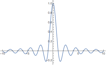
The (normalized) cardinal sine function sinc is defined by \[ \sinc(x) = \frac{\sin(\pi x)}{\pi x}, \quad x \in \R \] where it is understood that \( \sinc(0) = 1 \) (the limiting value).
If \( n \ge k \) then \( \E(Z^n) = \infty \). If \( 0 \le n \lt k \) then \[ \E(Z^n) = B\left(1 - \frac{n}{k}, 1 + \frac{n}{k}\right) = \frac{1}{\sinc(n / k)} \]
Using the PDF in , \[ \E(Z^n) = \int_0^\infty z^n \frac{k z^{k-1}}{(1 + z^k)^2} dz \] The substitution \( u = 1 / (1 + z^k) \), \( du = -k z^{k-1}/(1 + z^k)^2 \) gives \[ \E(Z^n) = \int_0^1 (1/u - 1)^{n/k} du = \int_0^1 u^{-n/k} (1 - u)^{n/k} du \] The result now follows from the definition of the beta function.
In particular, we can give the mean and variance.
If \( k \gt 1 \) then \[ \E(Z) = \frac{1}{\sinc(1/k)} \]
If \(k \gt 2 \) then \[ \var(Z) = \frac{1}{\sinc(2 / k)} - \frac{1}{\sinc^2(1 / k)} \]
Open the special distribution simulator and select the log-logistic distribution. Vary the shape parameter and note the size and location of the mean \( \pm \) standard deviation bar. For selected values of the shape parameter, run the simulation 1000 times and compare the empirical mean and standard deviation to the distribution mean and standard deviation.
The basic log-logistic distribution is preserved under power transformations.
If \( Z \) has the basic log-logistic distribution with shape parameter \( k \in (0, \infty) \) and if \( n \in (0, \infty) \), then \( W = Z^n \) has the basic log-logistic distribution with shape parameter \( k / n \).
For \( w \in [0, \infty) \), \[ \P(W \le w) = \P(Z \le w^{1/n}) = G\left(w^{1/n}\right) = \frac{w^{k/n}}{1 + w^{k/n}} \] As a function of \( w \), this is the CDF of the basic log-logistic distribution with shape parameter \( k/n \).
In particular, it follows that if \( V \) has the standard log-logistic distribution and \( k \in (0, \infty) \), then \( Z = V^{1/k} \) has the basic log-logistic distribution with shape parameter \( k \).
The log-logistic distribution has the usual connections with the standard uniform distribution by means of the distribution function in and the quantile function in .
Suppose that \( k \in (0, \infty) \).
Since the quantile function of the basic log-logistic distribution has a simple closed form, the distribution can be simulated using the random quantile method.
Open the random quantile experiment and select the log-logistic distribution. Vary the shape parameter and note the shape of the distribution and probability density functions. For selected values of the parameter, run the simulation 1000 times and compare the empirical density function, mean, and standard deviation to their distributional counterparts..
Of course, as mentioned in the introduction, the log-logistic distribution is related to the logistic distribution.
Suppose that \( k, \, b \in (0, \infty) \).
As a special case, (and as noted in the details of ), if \( Z \) has the standard log-logistic distribution, then \( Y = \ln Z \) has the standard logistic distribution, and if \( Y \) has the standard logistic distribution, then \( Z = e^Y \) has the standard log-logistic distribution.
The standard log-logistic distribution is the same as the standard beta prime distribution.
The PDF \(g\) of the standard log-logistic distribution is \( g(z) = 1 \big/ (1 + z)^2 \) for \( z \in [0, \infty) \), which is also the PDF of the standard beta prime distribution.
Of course, limiting distributions with respect to parameters are always interesting.
The basic log-logistic distribution with shape parameter \( k \in (0, \infty) \) converges to point mass at 1 as \( k \to \infty \).
We give two proofs.
The basic log-logistic distribution is generalized, like so many distributions on \( [0, \infty) \), by adding a scale parameter. Recall that a scale transformation often corresponds to a change of units (gallons into liters, for example), and so such transformations are of basic importance.
If \( Z \) has the basic log-logistic distribution with shape parameter \( k \in (0, \infty) \) and if \( b \in (0, \infty) \) then \( X = b Z \) has the log-logistic distribution with shape parameter \( k \) and scale parameter \( b \).
Suppose that \(X\) has the log-logistic distribution with shape parameter \(k \in (0, \infty)\) and scale parameter \(b \in (0, \infty)\).
\( X \) has distribution function \( F \) given by \[ F(x) = \frac{x^k}{b^k + x^k}, \quad x \in [0, \infty) \]
\( X \) has probability density function \( f \) given by \[ f(x) = \frac{b^k k x^{k-1}}{(b^k + x^k)^2}, \quad x \in (0, \infty) \] When \( k \ge 1 \), \( f \) is defined at 0 also. \( f \) satisfies the following properties:
Open the special distribution simulator and select the log-logistic distribution. Vary the shape and scale parameters and note the shape of the probability density function. For selected values of the parameters, run the simulation 1000 times and compare the empirical density function to the probability density function.
\( X \) has quantile function \( F^{-1} \) given by \[ F^{-1}(p) = b \left(\frac{p}{1 - p}\right)^{1/k}, \quad p \in [0, 1) \]
Open the quantile app and select the log-logistic distribution. Vary the shape and sclae parameters and note the shape of the distribution and probability density functions. For selected values of the parameters, compute the quantiles of order 0.1 and 0.9.
\( X \) has reliability function \( F^c \) given by \[ F^c(x) = \frac{b^k}{b^k + x^k}, \quad x \in [0, \infty) \]
The log-logistic distribution has either decreasing failure rate, or mixed decreasing-increasing failure rate, depending on the shape parameter.
\( X \) has failure rate function \( R \) given by \[ R(x) = \frac{k x^{k-1}}{b^k + x^k}, \quad x \in (0, \infty) \]
Suppose again that \( X \) has the log-logistic distribution with shape parameter \( k \in (0, \infty) \) and scale parameter \( b \in (0, \infty) \). The moments of \( X \) can be computed easily from the representation \( X = b Z \) where \( Z \) has the basic log-logistic distribution with shape parameter \( k \). Again, the expressions are simplest in terms of the beta function \( B \) and in terms of the normalized cardinal sine function sinc in .
If \( n \ge k \) then \( \E(X^n) = \infty \). If \( 0 \le n \lt k \) then \[ \E(X^n) = b^n B\left(1 - \frac{n}{k}, 1 + \frac{n}{k}\right) = \frac{b^n}{\sinc(n / k)} \]
If \( k \gt 1 \) then \[ \E(X) = \frac{b}{\sinc(1 / k)} \]
If \(k \gt 2 \) then \[ \var(X) = b^2 \left[\frac{1}{\sinc(2 / k)} - \frac{1}{\sinc^2(1 / k)} \right] \]
Open the special distribution simulator and select the log-logistic distribution. Vary the shape and scale parameters and note the size and location of the mean \(\pm\) standard deviation bar. For selected values of the parameters, run the simulation 1000 times compare the empirical mean and standard deviation to the distribution mean and standard deviation.
Since the log-logistic distribution is a scale family for each value of the shape parameter, it is trivially closed under scale transformations.
If \( X \) has the log-logistic distribution with shape parameter \( k \in (0, \infty) \) and scale parameter \( b \in (0, \infty) \), and if \( c \in (0, \infty) \), then \( Y = c X \) has the log-logistic distribution with shape parameter \( k \) and scale parameter \( b c \).
The log-logistic distribution is preserved under power transformations.
If \( X \) has the log-logistic distribution with shape parameter \( k \in (0, \infty) \) and scale parameter \( b \in (0, \infty) \), and if \( n \in (0, \infty) \), then \( Y = X^n \) has the log-logistic distribution with shape parameter \( k / n \) and scale parameter \( b^n \).
Again we can take \( X = b Z \) where \( Z \) has the basic log-logistic distribution with shape parameter \( k \). Then \( X^n = b^n Z^n \). But by , \( Z^n \) has the basic log-logistic distribution with shape parameter \( k / n \) and hence \( X \) has the log-logistic distribution with shape parameter \( k / n \) and scale parameter \( b^n \).
In particular, if \( V \) has the standard log-logistic distribution, then \( X = b V^{1 / k} \) has the log-logistic distribution with shape parameter \( k \) and scale parameter \( b \).
As before, the log-logistic distribution has the usual connections with the standard uniform distribution by means of the distribution function in and the quantile function in .
Suppose that \( k, \, b \in (0, \infty) \).
Again, since the quantile function of the log-logistic distribution has a simple closed form, the distribution can be simulated using the random quantile method.
Open the random quantile experiment and select the log-logistic distribution. Vary the shape and scale parameters and note the shape and location of the distribution and probability density functions. For selected values of the parameters, run the simulation 1000 times and compare the empirical density function, mean and standard deviation to their distributional counterparts.
Again, the logarithm of a log-logistic variable has the logistic distribution.
Suppose that \( k, \, b, \, c \in (0, \infty) \) and \( a \in \R \).
Once again, the limiting distribution is also of interest.
For fixed \( b \in (0, \infty) \), the log-logistic distribution with shape parameter \( k \in (0, \infty) \) and scale parameter \( b \) converges to point mass at \( b \) as \( k \to \infty \).
If \( X \) has the log-logistic distribution with shape parameter \( k \) and scale parameter \( b \), then as usual, we can write \( X = b Z \) where \( Z \) has the basic log-logistic distribution with shape parameter \( k \). From , we know that the distribution of \( Z \) converges to point mass at 1 as \( k \to \infty \), so it follows by the continuity theorem that the distribution of \( X \) converges to point mass at \( b \) as \( k \to \infty \).