Recall that by taking the expected value of various transformations of a random variable, we can measure many interesting characteristics of the distribution of the variable. In this section, we will study an expected value that measures a special type of relationship between two real-valued variables. This relationship is very important both in probability and statistics.
As usual, our starting point is a random experiment, modeled by a probability space \((\Omega, \mathscr F, \P)\). Unless otherwise noted, we assume that all expected values mentioned in this section exist. Suppose now that \(X\) and \(Y\) are real-valued random variables for the experiment (that is, defined on the probability space) with means \(\E(X)\), \(\E(Y)\), and variances \(\var(X)\), \(\var(Y)\), respectively.
The covariance of \((X, Y)\) is defined by \[ \cov(X, Y) = \E\left(\left[X - \E(X)\right]\left[Y - \E(Y)\right]\right) \] and, assuming the variances are positive, the correlation of \( (X, Y)\) is defined by \[ \cor(X, Y) = \frac{\cov(X, Y)}{\sd(X) \sd(Y)} \]
Correlation is a scaled version of covariance; note that the two parameters always have the same sign (positive, negative, or 0). Note also that correlation is dimensionless, since the numerator and denominator have the same physical units, namely the product of the units of \(X\) and \(Y\).
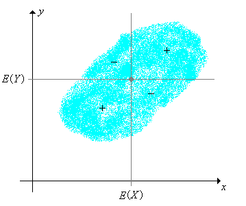
As these terms suggest, covariance and correlation measure a certain kind of dependence between the variables. One of our goals is a deeper understanding of this dependence. As a start, note that \(\left(\E(X), \E(Y)\right)\) is the center of the joint distribution of \((X, Y)\), and the vertical and horizontal lines through this point separate \(\R^2\) into four quadrants. The function \((x, y) \mapsto \left[x - \E(X)\right]\left[y - \E(Y)\right]\) is positive on the first and third quadrants and negative on the second and fourth.
The following theorems give some basic properties of covariance. The main tool that we will need is the fact that expected value is a linear operation. Other important properties will be derived below, in the subsection on the best linear predictor. As usual, be sure to try the proofs yourself before reading details. Once again, we assume that the random variables are defined on the common sample space, are real-valued, and that the indicated expected values exist (as real numbers).
Our first result is a formula that is better than the definition for computational purposes, but gives less insight.
\(\cov(X, Y) = \E(X Y) - \E(X) \E(Y)\).
Let \( \mu = \E(X) \) and \( \nu = \E(Y) \). Then \[ \cov(X, Y) = \E\left[(X - \mu)(Y - \nu)\right] = \E(X Y - \mu Y - \nu X + \mu \nu) = \E(X Y) - \mu \E(Y) - \nu \E(X) + \mu \nu = \E(X Y) - \mu \nu \]
From , we see that \(X\) and \(Y\) are uncorrelated if and only if \(\E(X Y) = \E(X) \E(Y)\), so here is a simple but important corollary for independent variables.
If \(X\) and \(Y\) are independent, then they are uncorrelated.
We showed in the section on basic properties that if \(X\) and \(Y\) are indepedent then \(\E(X Y) = \E(X) \E(Y)\).
However, the converse fails with a passion: Exercise gives an example of two variables that are functionally related (the strongest form of dependence), yet uncorrelated. The computational exercises give other examples of dependent yet uncorrelated variables also. Note also that if one of the variables has mean 0, then the covariance is simply the expected product.
Trivially, covariance is a symmetric operation.
\(\cov(X, Y) = \cov(Y, X)\).
As the name suggests, covariance generalizes variance.
\(\cov(X, X) = \var(X)\).
Let \( \mu = \E(X) \). Then \( \cov(X, X) = \E\left[(X - \mu)^2\right] = \var(X) \).
Covariance is a linear operation in the first argument, if the second argument is fixed.
If \(X\), \(Y\), \(Z\) are random variables, and \(c\) is a constant, then
By symmetry, covariance is also a linear operation in the second argument, with the first argument fixed. Thus, the covariance operator is bi-linear. The general version of this property is given in :
Suppose that \((X_1, X_2, \ldots, X_n)\) and \((Y_1, Y_2, \ldots, Y_m)\) are sequences of random variables, and that \((a_1, a_2, \ldots, a_n)\) and \((b_1, b_2, \ldots, b_m)\) are constants. Then \[ \cov\left(\sum_{i=1}^n a_i \, X_i, \sum_{j=1}^m b_j \, Y_j\right) = \sum_{i=1}^n \sum_{j=1}^m a_i \, b_j \, \cov(X_i, Y_j) \]
Proposition given next shows how covariance is changed under a linear transformation of one of the variables. This is simply a special case of the basic properties, but is worth stating.
If \( a, \, b \in \R \) then \(\cov(a + bX, Y) = b \, \cov(X, Y)\).
A constant is independent of any random variable. Hence \( \cov(a + b X, Y) = \cov(a, Y) + b \, \cov(X, Y) = b \, \cov(X, Y) \).
Of course, by symmetry, the same property holds in the second argument. Putting the two together we have that if \( a, \, b, \, c, \, d \in \R \) then \( \cov(a + b X, c + d Y) = b d \, \cov(X, Y) \).
Next we will establish some basic properties of correlation. Most of these follow easily from corresponding properties of covariance above. We assume that \(\var(X) \gt 0\) and \(\var(Y) \gt 0\), so that the random variable really are random and hence the correlation is well defined. For the first result, recall the definition of the standard score of a variable.
The correlation between \(X\) and \(Y\) is the covariance of the corresponding standard scores: \[ \cor(X, Y) = \cov\left(\frac{X - \E(X)}{\sd(X)}, \frac{Y - \E(Y)}{\sd(Y)}\right) = \E\left(\frac{X - \E(X)}{\sd(X)} \frac{Y - \E(Y)}{\sd(Y)}\right) \]
From the definitions and the linearity of expected value, \[ \cor(X, Y) = \frac{\cov(X, Y)}{\sd(X) \sd(Y)} = \frac{\E\left(\left[X - \E(X)\right]\left[Y - \E(Y)\right]\right)}{\sd(X) \sd(Y)} = \E\left(\frac{X - \E(X)}{\sd(X)} \frac{Y - \E(Y)}{\sd(Y)}\right) \] Since the standard scores have mean 0, this is also the covariance of the standard scores.
This shows again that correlation is dimensionless, since of course, the standard scores are dimensionless. Also, correlation is symmetric:
\(\cor(X, Y) = \cor(Y, X)\).
Under a linear transformation of one of the variables, the correlation is unchanged if the slope is positve and changes sign if the slope is negative:
If \(a, \, b \in \R\) and \( b \ne 0 \) then
This result reinforces the fact that correlation is a standardized measure of association, since multiplying the variable by a positive constant is equivalent to a change of scale, and adding a contant to a variable is equivalent to a change of location. For example, in the Challenger data, the underlying variables are temperature at the time of launch (in degrees Fahrenheit) and O-ring erosion (in millimeters). The correlation between these two variables is of fundamental importance. If we decide to measure temperature in degrees Celsius and O-ring erosion in inches, the correlation is unchanged. Of course, the same property holds in the second argument, so if \( a, \, b, \, c, \, d \in \R \) with \( b \ne 0 \) and \( d \ne 0 \), then \( \cor(a + b X, c + d Y) = \cor(X, Y) \) if \( b d \gt 0 \) and \( \cor(a + b X, c + d Y) = -\cor(X, Y) \) if \( b d \lt 0 \).
The most important properties of covariance and correlation will emerge from our study of the best linear predictor below.
We will now show that the variance of a sum of variables is the sum of the pairwise covariances. This result is very useful since many random variables with special distributions can be written as sums of simpler random variables (see in particular the binomial distribution in and hypergeometric distribution in ).
If \((X_1, X_2, \ldots, X_n)\) is a sequence of real-valued random variables then \[ \var\left(\sum_{i=1}^n X_i\right) = \sum_{i=1}^n \sum_{j=1}^n \cov(X_i, X_j) = \sum_{i=1}^n \var(X_i) + 2 \sum_{\{(i, j): i \lt j\}} \cov(X_i, X_j) \]
From and , \[ \var\left(\sum_{i=1}^n X_i\right) = \cov\left(\sum_{i=1}^n X_i, \sum_{j=1}^n X_j\right) = \sum_{i=1}^j \sum_{j=1}^n \cov(X_i, X_j) \] The second expression follows since \( \cov(X_i, X_i) = \var(X_i) \) for each \( i \) and \( \cov(X_i, X_j) = \cov(X_j, X_i) \) for \( i \ne j \) by the symmetry property .
Note that the variance of a sum can be larger, smaller, or equal to the sum of the variances, depending on the pure covariance terms. As a special case of , when \(n = 2\), we have \[ \var(X + Y) = \var(X) + \var(Y) + 2 \, \cov(X, Y) \] The following corollary is very important.
If \((X_1, X_2, \ldots, X_n)\) is a sequence of pairwise uncorrelated, real-valued random variables then \[ \var\left(\sum_{i=1}^n X_i\right) = \sum_{i=1}^n \var(X_i) \]
Note that the last result holds, in particular, if the random variables are independent. We close this discussion with a couple of minor corollaries.
If \(X\) and \(Y\) are real-valued random variables then \(\var(X + Y) + \var(X - Y) = 2 \, [\var(X) + \var(Y)]\).
If \(X\) and \(Y\) are real-valued random variables with \(\var(X) = \var(Y)\) then \(X + Y\) and \(X - Y\) are uncorrelated.
In the following exercises, suppose that \((X_1, X_2, \ldots)\) is a sequence of independent, real-valued random variables with a common distribution that has mean \(\mu\) and standard deviation \(\sigma \gt 0\). In statistical terms, the variables form a random sample from the common distribution.
For \(n \in \N+\), let \(Y_n = \sum_{i=1}^n X_i\).
For \(n \in \N_+\), let \(M_n = Y_n \big/ n = \frac{1}{n} \sum_{i=1}^n X_i\), so that \(M_n\) is the sample mean of \((X_1, X_2, \ldots, X_n)\).
Part (c) of means that \(M_n \to \mu\) as \(n \to \infty\) in mean square. Part (d) means that \(M_n \to \mu\) as \(n \to \infty\) in probability. These are both versions of the law of large numbers, one of the fundamental theorems of probability.
The standard score of the sum \( Y_n \) and the standard score of the sample mean \( M_n \) are the same: \[ Z_n = \frac{Y_n - n \, \mu}{\sqrt{n} \, \sigma} = \frac{M_n - \mu}{\sigma / \sqrt{n}} \]
The equality of the standard score of \( Y_n \) and of \( Z_n \) is a result of simple algebra. But recall more generally that the standard score of a variable is unchanged by a linear transformation of the variable with positive slope (a location-scale transformation of the distribution). Of course, parts (a) and (b) are true for any standard score.
The central limit theorem, the other fundamental theorem of probability, states that the distribution of \(Z_n\) converges to the standard normal distribution as \(n \to \infty\).
If \(A\) and \(B\) are events in our random experiment then the covariance and correlation of \(A\) and \(B\) are defined to be the covariance and correlation, respectively, of their indicator random variables.
If \(A\) and \(B\) are events, define \(\cov(A, B) = \cov(\bs 1_A, \bs 1_B)\) and \(\cor(A, B) = \cor(\bs 1_A, \bs 1_B)\). Equivalently,
Recall that if \( X \) is an indicator variable with \( \P(X = 1) = p \), then \( \E(X) = p \) and \( \var(X) = p (1 - p) \). Also, if \( X \) and \( Y \) are indicator variables then \( X Y \) is an indicator variable and \( \P(X Y = 1) = \P(X = 1, Y = 1) \). The results then follow from the definitions.
In particular, note that \(A\) and \(B\) are positively correlated, negatively correlated, or independent, respectively (as defined in the section on conditional probability) if and only if the indicator variables of \(A\) and \(B\) are positively correlated, negatively correlated, or uncorrelated, as defined in .
If \(A\) and \(B\) are events then
If \( A \) and \( B \) are events with \(A \subseteq B\) then
In the language of the experiment, \( A \subseteq B \) means that \( A \) implies \( B \). In such a case, the events are positively correlated, not surprising.
What linear function of \(X\) (that is, a function of the form \( a + b X \) where \( a, \, b \in \R \)) is closest to \(Y\) in the sense of minimizing mean square error? The question is fundamentally important in the case where random variable \(X\) (the predictor variable) is observable and random variable \(Y\) (the response variable) is not. The linear function can be used to estimate \(Y\) from an observed value of \(X\). Moreover, the solution will have the added benefit of showing that covariance and correlation measure the linear relationship between \(X\) and \(Y\). To avoid trivial cases, let us assume that \(\var(X) \gt 0\) and \(\var(Y) \gt 0\), so that the random variables really are random. The solution to our problem turns out to be the linear function of \( X \) with the same expected value as \( Y \), and whose covariance with \( X \) is the same as that of \( Y \).
The random variable \(L(Y \mid X)\) defined as follows is the only linear function of \(X\) satisfying properties (a) and (b). \[ L(Y \mid X) = \E(Y) + \frac{\cov(X, Y)}{\var(X)} \left[X - \E(X)\right] \]
By the linearity of expected value, \[ \E\left[L(Y \mid X)\right] = \E(Y) + \frac{\cov(X, Y)}{\var(X)} \left[\E(X) - \E(X)\right] = \E(Y) \] Next, by the linearity of covariance and the fact that a constant is independent (and hence uncorrelated) with any random variable, \[ \cov\left[X, L(Y \mid X)\right] = \frac{\cov(X, Y)}{\var(X)} \cov(X, X) = \frac{\cov(X, Y)}{\var(X)} \var(X) = \cov(X, Y) \] Conversely, suppose that \( U = a + b X \) satisfies \(\E(U) = \E(Y)\) and \( \cov(X, U) = \cov(Y, U) \). Again using linearity of covariance and the uncorrelated property of constants, the second equation gives \( b \, \cov(X, X) = \cov(X, Y) \) so \( b = \cov(X, Y) \big/ \var(X) \). Then the first equation gives \( a = \E(Y) - b \E(X) \), so \( U = L(Y \mid X) \).
Note that in the presence of part (a), part (b) is equivalent to \( \E\left[X L(Y \mid X)\right] = \E(X Y) \). Here is another minor variation, but one that will be very useful: \( L(Y \mid X) \) is the only linear function of \( X \) with the same mean as \( Y \) and with the property that \( Y - L(Y \mid X) \) is uncorrelated with every linear function of \( X \).
\( L(Y \mid X) \) is the only linear function of \( X \) that satisfies
Of course part (a) is the same as part (a) of . Suppose that \( U = a + b X \) where \( a, \, b \in \R \). From basic properties of covariance and the previous result, \[ \cov\left[Y - L(Y \mid X), U\right] = b \, \cov\left[Y - L(Y \mid X), X\right] = b \left(\cov(Y, X) - \cov\left[L(Y \mid X), X\right]\right) = 0 \] Conversely, suppose that \( V \) is a linear function of \( X \) and that \( \E(V) = \E(Y) \) and \( \cov(Y - V, U) = 0 \) for every linear function \( U \) of \( X \). Letting \( U = X \) we have \( \cov(Y - V, X) = 0 \) so \( \cov(V, X) = \cov(Y, X) \). Hence \( V = L(Y \mid X) \) by .
The variance of \( L(Y \mid X) \) and its covariance with \( Y \) turn out to be the same.
Additional properties of \( L(Y \mid X) \):
We can now prove the fundamental result that \( L(Y \mid X) \) is the linear function of \( X \) that is closest to \( Y \) in the mean square sense. We give two proofs; the first is more straightforward, but the second is more interesting and elegant.
Suppose that \( U \) is a linear function of \( X \). Then
Our first proof uses calculus. Let \(\mse(a, b)\) denote the mean square error when \(U = a + b \, X\) is used as an estimator of \(Y\), as a function of the parameters \(a, \, b \in \R\): \[ \mse(a, b) = \E\left(\left[Y - (a + b \, X)\right]^2 \right) \] Expanding the square and using the linearity of expected value gives \[ \mse(a, b) = a^2 + b^2 \E(X^2) + 2 a b \E(X) - 2 a \E(Y) - 2 b \E(X Y) + \E(Y^2) \] In terms of the variables \( a \) and \( b \), the first three terms are the second-order terms, the next two are the first-order terms, and the last is the zero-order term. The second-order terms define a quadratic form whose standard symmetric matrix is \[ \left[\begin{matrix} 1 & \E(X) \\ \E(X) & \E(X^2) \end{matrix} \right]\] The determinant of this matrix is \( \E(X^2) - [\E(X)]^2 = \var(X) \) and the diagonal terms are positive. All of this means that the graph of \( \mse \) is a paraboloid opening upward, so the minimum of \( \mse \) will occur at the unique critical point. Setting the first derivatives of \( \mse \) to 0 we have \begin{align} -2 \E(Y) + 2 b \E(X) + 2 a & = 0 \\ -2 \E(X Y) + 2 b \E\left(X^2\right) + 2 a \E(X) & = 0 \end{align} Solving the first equation for \( a \) gives \( a = \E(Y) - b \E(X) \). Substituting this into the second equation and solving gives \( b = \cov(X, Y) \big/ \var(X) \).
Our second proof uses basic properties.
The mean square error when \( L(Y \mid X) \) is used as a predictor of \( Y \) is \[ \E\left(\left[Y - L(Y \mid X)\right]^2 \right) = \var(Y)\left[1 - \cor^2(X, Y)\right] \]
Again, let \( L = L(Y \mid X) \) for convenience. Since \( Y - L \) has mean 0, \[ \E\left[(Y - L)^2\right] = \var(Y - L) = \var(Y) - 2 \cov(L, Y) + \var(L) \] But \( \cov(L, Y) = \var(L) = \cov^2(X, Y) \big/ \var(X) \) by . Hence \[ \E\left[(Y - L)^2\right] = \var(Y) - \frac{\cov^2(X, Y)}{\var(X)} = \var(Y) \left[1 - \frac{\cov^2(X, Y)}{\var(X) \var(Y)}\right] = \var(Y) \left[1 - \cor^2(X, Y)\right] \]
Our solution to the best linear perdictor problems yields important properties of covariance and correlation.
Additional properties of covariance and correlation:
Since mean square error is nonnegative, it follows from that \(\cor^2(X, Y) \le 1\). This gives parts (a) and (b). For parts (c) and (d), note that if \(\cor^2(X, Y) = 1\) then \(Y = L(Y \mid X)\) with probability 1, and that the slope in \( L(Y \mid X) \) has the same sign as \( \cor(X, Y) \).
The last two results clearly show that \(\cov(X, Y)\) and \(\cor(X, Y)\) measure the linear association between \(X\) and \(Y\). The equivalent inequalities (a) and (b) above are referred to as the correlation inequality. They are also versions of the Cauchy-Schwarz inequality, named for Augustin Cauchy and Karl Schwarz
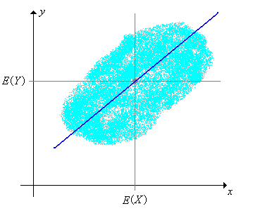
Recall that the best constant predictor of \(Y\), in the sense of minimizing mean square error, is \(\E(Y)\) and the minimum value of the mean square error for this predictor is \(\var(Y)\). Thus, the difference between the variance of \(Y\) and the mean square error for \( L(Y \mid X) \) is the reduction in the variance of \(Y\) when the linear term in \(X\) is added to the predictor: \[\var(Y) - \E\left(\left[Y - L(Y \mid X)\right]^2\right) = \var(Y) \, \cor^2(X, Y)\] So \(\cor^2(X, Y)\) is the proportion of reduction in \(\var(Y)\) when \(X\) is included as a predictor variable. This quantity is called the (distribution) coefficient of determination. Now let \[ L(Y \mid X = x) = \E(Y) + \frac{\cov(X, Y)}{\var(X)}\left[x - \E(X)\right], \quad x \in \R \] The function \(x \mapsto L(Y \mid X = x)\) is known as the distribution regression function for \(Y\) given \(X\), and its graph is known as the distribution regression line. Note that the regression line passes through \(\left(\E(X), \E(Y)\right)\), the center of the joint distribution.
However, the choice of predictor variable and response variable is crucial.
The regression line for \(Y\) given \(X\) and the regression line for \(X\) given \(Y\) are not the same line, except in the trivial case where the variables are perfectly correlated. However, the coefficient of determination is the same, regardless of which variable is the predictor and which is the response.
The two regression lines are \begin{align} y - \E(Y) & = \frac{\cov(X, Y)}{\var(X)}\left[x - \E(X)\right] \\ x - \E(X) & = \frac{\cov(X, Y)}{\var(Y)}\left[y - \E(Y)\right] \end{align} The two lines are the same if and only if \( \cov^2(X, Y) = \var(X) \var(Y) \). But this is equivalent to \( \cor^2(X, Y) = 1 \).
Suppose that \(A\) and \(B\) are events with \(0 \lt \P(A) \lt 1\) and \(0 \lt \P(B) \lt 1\). Then
Recall from that \(\cor(A, B) = \cor(\bs 1_A, \bs 1_B)\), so if \(\cor^2(A, B) = 1\) then from , \(\bs 1_B = L(\bs 1_B \mid \bs 1_A)\) with probability 1. But \(\bs 1_A\) and \(\bs 1_B\) each takes values 0 and 1 only. Hence the only possible regression lines are \(y = 0\), \(y = 1\), \(y = x\) and \(y = 1 - x\). The first two correspond to \(\P(B) = 0\) and \(\P(B) = 1\), respectively, which are excluded by the hypotheses.
The concept of best linear predictor is more powerful than might first appear, because it can be applied to transformations of the variables. Specifically, suppose that \(X\) and \(Y\) are random variables for our experiment, taking values in general spaces \(S\) and \(T\), respectively. Suppose also that \(g\) and \(h\) are real-valued functions defined on \(S\) and \(T\), respectively. We can find \(L\left[h(Y) \mid g(X)\right]\), the linear function of \(g(X)\) that is closest to \(h(Y)\) in the mean square sense. The results of this subsection apply, of course, with \(g(X)\) replacing \(X\) and \(h(Y)\) replacing \(Y\). Of course, we must be able to compute the appropriate means, variances, and covariances.
We close this subsection with two additional properties of the best linear predictor, the linearity properties. Once again, the details give two proofs.
Suppose that \( X \), \( Y \), and \(Z\) are random variables and that \(c\) is a constant. Then
Our first proof is uses the definitions. The results follow easily from the linearity of expected value and covariance.
Our second proof uses the characterizing properties:
There are several extensions and generalizations of the ideas in the subsection:
The use of characterizing properties will play a crucial role in these extensions.
Suppose that \(X\) is uniformly distributed on the interval \([-1, 1]\) and \(Y = X^2\). Then \(X\) and \(Y\) are uncorrelated even though \(Y\) is a function of \(X\) (the strongest form of dependence).
Note that \( \E(X) = 0 \) and \( \E(Y) = \E\left(X^2\right) = 1 / 3 \) and \( \E(X Y) = E\left(X^3\right) = 0 \). Hence \( \cov(X, Y) = \E(X Y) - \E(X) \E(Y) = 0 \).
Suppose that \((X, Y)\) is uniformly distributed on the region \(S \subseteq \R^2\). Find \(\cov(X, Y)\) and \(\cor(X, Y)\) and determine whether the variables are independent in each of the following cases:
In the bivariate uniform experiment, select each of the regions below in turn. For each region, run the simulation 2000 times and note the value of the correlation and the shape of the cloud of points in the scatterplot. Compare with the results in .
Suppose that \(X\) is uniformly distributed on the interval \((0, 1)\) and that given \(X = x \in (0, 1)\), \(Y\) is uniformly distributed on the interval \((0, x)\). Find each of the following:
Recall that a standard die is a six-sided die. A fair die is one in which the faces are equally likely. An ace-six flat die is a standard die in which faces 1 and 6 have probability \(\frac{1}{4}\) each, and faces 2, 3, 4, and 5 have probability \(\frac{1}{8}\) each.
A pair of standard, fair dice are thrown and the scores \((X_1, X_2)\) recorded. Let \(Y = X_1 + X_2\) denote the sum of the scores, \(U = \min\{X_1, X_2\}\) the minimum scores, and \(V = \max\{X_1, X_2\}\) the maximum score. Find the covariance and correlation of each of the following pairs of variables:
Suppose that \(n\) fair dice are thrown. Find the mean and variance of each of the following variables:
In the dice experiment, select fair dice, and select the following random variables. In each case, increase the number of dice and observe the size and location of the probability density function and the mean \( \pm \) standard deviation bar. With \(n = 20\) dice, run the experiment 1000 times and compare the sample mean and standard deviation to the distribution mean and standard deviation.
Suppose that \(n\) ace-six flat dice are thrown. Find the mean and variance of each of the following variables:
In the dice experiment, select ace-six flat dice, and select the following random variables. In each case, increase the number of dice and observe the size and location of the probability density function and the mean \( \pm \) standard deviation bar. With \(n = 20\) dice, run the experiment 1000 times and compare the sample mean and standard deviation to the distribution mean and standard deviation.
A pair of fair dice are thrown and the scores \((X_1, X_2)\) recorded. Let \(Y = X_1 + X_2\) denote the sum of the scores, \(U = \min\{X_1, X_2\}\) the minimum score, and \(V = \max\{X_1, X_2\}\) the maximum score. Find each of the following:
Recall that a Bernoulli trials process is a sequence \(\boldsymbol{X} = (X_1, X_2, \ldots)\) of independent, identically distributed indicator random variables. In the usual language of reliability, \(X_i\) denotes the outcome of trial \(i\), where 1 denotes success and 0 denotes failure. The probability of success \(p = \P(X_i = 1)\) is the basic parameter of the process. The process is named for Jacob Bernoulli.
For \(n \in \N_+\), the number of successes in the first \(n\) trials is \(Y_n = \sum_{i=1}^n X_i\). Recall that this random variable has the binomial distribution with parameters \(n\) and \(p\), which has probability density function \(f\) given by \[ f_n(y) = \binom{n}{y} p^y (1 - p)^{n - y}, \quad y \in \{0, 1, \ldots, n\} \]
The mean and variance of \(Y_n\) are
In the binomial coin experiment, select the number of heads. Vary \(n\) and \(p\) and note the shape of the probability density function and the size and location of the mean \( \pm \) standard deviation bar. For selected values of the parameters, run the experiment 1000 times and compare the sample mean and standard deviation to the distribution mean and standard deviation.
For \(n \in \N_+\), the proportion of successes in the first \(n\) trials is \(M_n = Y_n / n\). This random variable is sometimes used as a statistical estimator of the parameter \(p\), when the parameter is unknown.
The mean and variance of \(M_n\) are
In the binomial coin experiment, select the proportion of heads. Vary \(n\) and \(p\) and note the shape of the probability density function and the size and location of the mean \( \pm \) standard deviation bar. For selected values of the parameters, run the experiment 1000 times and compare the sample mean and standard deviation to the distribution mean and standard deviation.
As a special case of note that \(M_n \to p\) as \(n \to \infty\) in mean square and in probability.
Suppose that a population consists of \(m\) objects; \(r\) of the objects are type 1 and \(m - r\) are type 0. A sample of \(n\) objects is chosen at random, without replacement. The parameters \(m, \, n \in \N_+\) and \(r \in \N\) with \(n \le m\) and \(r \le m\). For \(i \in \{1, 2, \ldots, n\}\), let \(X_i\) denote the type of the \(i\)th object selected. Recall that \((X_1, X_2, \ldots, X_n)\) is a sequence of identically distributed (but not independent) indicator random variables.
Let \(Y\) denote the number of type 1 objects in the sample, so that \(Y = \sum_{i=1}^n X_i\). Recall that this random variable has the hypergeometric distribution, which has probability density function \(f_n\) given by \[ f(y) = \frac{\binom{r}{y} \binom{m - r}{n - y}}{\binom{m}{n}}, \quad y \in \{0, 1, \ldots, n\} \]
For distinct \(i, \, j \in \{1, 2, \ldots, n\}\),
Recall that \( \E(X_i) = \P(X_i = 1) = \frac{r}{m} \) for each \( i \) and \( \E(X_i X_j) = \P(X_i = 1, X_j = 1) = \frac{r}{m} \frac{r - 1}{m - 1} \) for each \( i \ne j \). Technically, the sequence of indicator variables is exchangeable. The results now follow from the definitions and simple algebra.
Note that the event of a type 1 object on draw \(i\) and the event of a type 1 object on draw \(j\) are negatively correlated, but the correlation depends only on the population size and not on the number of type 1 objects. Note also that the correlation is perfect if \(m = 2\). Think about these result intuitively.
The mean and variance of \(Y\) are
Note that if the sampling were with replacement, \( Y \) would have a binomial distribution, and so in particular \( E(Y) = n \frac{r}{m} \) and \( \var(Y) = n \frac{r}{m} \left(1 - \frac{r}{m}\right) \). The additional factor \( \frac{m - n}{m - 1} \) that occurs in the variance of the hypergeometric distribution is sometimes called the finite population correction factor. Note that for fixed \( m \), \( \frac{m - n}{m - 1} \) is decreasing in \( n \), and is 0 when \( n = m \). Of course, we know that we must have \( \var(Y) = 0 \) if \( n = m \), since we would be sampling the entire population, and so deterministically, \( Y = r \). On the other hand, for fixed \( n \), \( \frac{m - n}{m - 1} \to 1\) as \( m \to \infty \). More generally, the hypergeometric distribution is well approximated by the binomial when the population size \( m \) is large compared to the sample size \( n \).
In the ball and urn experiment, select sampling without replacement. Vary \(m\), \(r\), and \(n\) and note the shape of the probability density function and the size and location of the mean \( \pm \) standard deviation bar. For selected values of the parameters, run the experiment 1000 times and compare the sample mean and standard deviation to the distribution mean and standard deviation.
Suppose that \(X\) and \(Y\) are real-valued random variables with \(\cov(X, Y) = 3\). Find \(\cov(2 X - 5, 4 Y + 2)\).
24
Suppose \(X\) and \(Y\) are real-valued random variables with \(\var(X) = 5\), \(\var(Y) = 9\), and \(\cov(X, Y) = - 3\). Find
Suppose that \(X\) and \(Y\) are independent, real-valued random variables with \(\var(X) = 6\) and \(\var(Y) = 8\). Find \(\var(3 X - 4 Y + 5)\).
182
Suppose that \(A\) and \(B\) are events in an experiment with \(\P(A) = \frac{1}{2}\), \(\P(B) = \frac{1}{3}\), and \(\P(A \cap B) = \frac{1}{8}\). Find each of the following:
Suppose that \( X \), \( Y \), and \( Z \) are real-valued random variables for an experiment, and that \( L(Y \mid X) = 2 - 3 X \) and \( L(Z \mid X) = 5 + 4 X \). Find \( L(6 Y - 2 Z \mid X) \).
\( 2 - 26 X \)
Suppose that \( X \) and \( Y \) are real-valued random variables for an experiment, and that \( \E(X) = 3 \), \( \var(X) = 4 \), and \( L(Y \mid X) = 5 - 2 X \). Find each of the following:
Suppose that \((X, Y)\) has probability density function \(f\) given by \(f(x, y) = x + y\) for \(0 \le x \le 1\), \(0 \le y \le 1\). Find each of the following
Suppose that \((X, Y)\) has probability density function \(f\) given by \(f(x, y) = 2 (x + y)\) for \(0 \le x \le y \le 1\). Find each of the following:
Suppose again that \((X, Y)\) has probability density function \(f\) given by \(f(x, y) = 2 (x + y)\) for \(0 \le x \le y \le 1\).
Suppose that \((X, Y)\) has probability density function \(f\) given by \(f(x, y) = 6 x^2 y\) for \(0 \le x \le 1\), \(0 \le y \le 1\). Find each of the following:
Note that \(X\) and \(Y\) are independent.
Suppose that \((X, Y)\) has probability density function \(f\) given by \(f(x, y) = 15 x^2 y\) for \(0 \le x \le y \le 1\). Find each of the following:
Suppose again that \((X, Y)\) has probability density function \(f\) given by \(f(x, y) = 15 x^2 y\) for \(0 \le x \le y \le 1\).